Chapter 4

Subtasks

4.1. Equational reasoning

Equality chains are ubiquitous in mathematics. Here, by equality chain, I mean parts of proofs found in mathematical literature that consist of a list of expressions separated by = or some other transitive relation symbol. The chains are chosen such that each pair of adjacent expressions are clearly equal to the reader, in the sense that the equality does not need to be explicitly justified. And hence, by transitivity, the chain shows that the first expression is equal to the last one.

For example, take some vector space V. Suppose that one wishes to prove that given a linear map 𝐴 : V ⟶ V, its adjoint 𝐴† : V → V is linearIn general, the adjoint should act on the dual space 𝐴† : V* → V*.. To do so one typically provides the equality chain (4.1) for all vectors 𝑥 𝑢 𝑣 : V.

(4.1)

The running example problem for this chapter. Here, ⟨_, _⟩ : V × V → ℂ is the inner product taking a pair of vectors to a complex number.

⟨𝐴† (𝑢 + 𝑣), 𝑥⟩
  = ⟨𝑢 + 𝑣, 𝐴 𝑥⟩
  = ⟨𝑢, 𝐴 𝑥⟩ + ⟨𝑣, 𝐴 𝑥⟩
  = ⟨𝐴† 𝑢, 𝑥⟩ + ⟨𝑣, 𝐴 𝑥⟩
  = ⟨𝐴† 𝑢, 𝑥⟩ + ⟨𝐴† 𝑣, 𝑥⟩
  = ⟨𝐴† 𝑢 + 𝐴† 𝑣, 𝑥⟩

The equations that one can compose the reasoning chain from (e.g., ⟨𝐴† 𝑎, 𝑏⟩ = ⟨𝑎, 𝐴 𝑏⟩) are called rewrite rules. For the example (4.1), there are a large number of axiomatic rewrite rules available (4.2) and still more rules derived from these. We can formulate the equation rewriting problem for two expressions Γ ⊢ 𝑙 = 𝑟 as finding a path in the graph E whose vertices are expressions in Γ and whose edges are generated by a set of rewrite rules 𝑅 (such as those in (4.2)). Any free variables in 𝑅 are substituted with correctly typed expressions to produce ground rewrite rules that are then closed under symmetry, transitivity, congruenceA relation ~ is congruent when 𝑥 ~ 𝑦 implies 𝑡⦃𝑧 ↦ 𝑥⦄ ~ 𝑡⦃𝑧 ↦ 𝑦⦄ for all valid expressions 𝑥, 𝑦 and 𝑡 where 𝑡 has a free variable 𝑧..

(4.2)

A possible set of rewrite rules relevant to (4.1). Where 𝑎 𝑏 𝑐 : ℂ for some field ℂ; 𝑥 𝑦 𝑧 : V for some ℂ-vector space V; and A : V ⟶ V is a linear map in V. Note that the vector space laws are over an arbitrary vector space and so can also apply to the dual space V. This list is for illustrative purposes rather than being exhaustive: the details within an ITP can vary. For example, in Lean, there is a single commutativity rule ∀ (𝑎 𝑏 : α) [comm_monoid α], 𝑎 * 𝑏 = 𝑏 * 𝑎 which applies to any type with an instance of the comm_monoid typeclass.

𝑎 + 𝑏 = 𝑏 + 𝑎

𝑎 + (𝑏 + 𝑐) = (𝑎 + 𝑏) + 𝑐

0 + 𝑎 = 𝑎

𝑎 + - 𝑎 = 0

- 𝑎 + 𝑎 = 0

𝑎 * 𝑏 = 𝑏 * 𝑎

𝑎 * (𝑏 * 𝑐) = (𝑎 * 𝑏) * 𝑐

1 * 𝑎 = 𝑎

𝑎 ≠ 0 → 𝑎 * 𝑎⁻¹ = 1

𝑎 ≠ 0 → 𝑎⁻¹ * 𝑎 = 1

𝑎 * (𝑏 + 𝑐) = 𝑎 * 𝑏 + 𝑎 * 𝑐

𝑦 + 𝑥 = 𝑥 + 𝑦

𝑥 + (𝑦 + 𝑧) = (𝑥 + 𝑦) + 𝑧

𝑥 + 0 = 0

1 • 𝑥 = 𝑥

(𝑎 + 𝑏) • 𝑥 = 𝑎 • 𝑥 + 𝑏 • 𝑥

(𝑎 * 𝑏) • 𝑥 = 𝑎 • (𝑏 • 𝑥)

𝑎 • (𝑥 + 𝑦) = 𝑎 • 𝑥 + 𝑎 • 𝑦

⟨𝑢 + 𝑣, 𝑥⟩ = ⟨𝑢, 𝑥⟩ + ⟨𝑣, 𝑥⟩

⟨𝑢, 𝑥 + 𝑦⟩ = ⟨𝑢, 𝑥⟩ + ⟨𝑢, 𝑦⟩

𝑎 * ⟨𝑢, 𝑥⟩ = ⟨𝑎 • 𝑢, 𝑥⟩

𝑎 * ⟨𝑢, 𝑥⟩ = ⟨𝑢, 𝑎 • 𝑥⟩

𝐴 (𝑥 + 𝑦) = 𝐴 𝑥 + 𝐴 𝑦

𝑎 • 𝐴 𝑥 = 𝐴 (𝑎 • 𝑥)

⟨𝐴† 𝑢, 𝑥⟩ = ⟨𝑢, 𝐴 𝑥⟩

A central part of automated theorem proving (ATP) is constructing equality proofs such as (4.1) from (4.2) automatically. This can be done with well-researched techniques from the field of term rewriting systems [BN98[BN98]Baader, Franz; Nipkow, TobiasTerm rewriting and all that (1998)publisher Cambridge University Presshttps://doi.org/10.1017/CBO9781139172752]. These techniques take advantage of the fact that computers can perform many operations per second, and large search spaces can be explored quickly, though heuristic functions are still needed to prevent a combinatorial explosion. Many domains - such as checking that two expressions are equal using the ring axioms - also have specialised decision procedures available for them. I'll call these approaches to solving equalities machine-oriented; this contrasts with human-oriented as discussed in Section 2.6.

In accordance with the research goals of this thesis (Section 1.2), the purpose here is to investigate alternative, human-like ways of producing equality proofs. As motivated in Section 1.1, this serves the purpose of improving the usability of proof assistants by making the proofs generated more understandable (Section 2.5). The goal of this chapter is not to develop methods that compete with machine-oriented techniques to prove more theorems or prove them faster. Instead, I want to focus on the abstract reasoning that a human mathematician typically carries out when they encounter an equality reasoning problem such as (4.1).

With this in mind, the goal of this chapter is to create an algorithm which:

can solve simple equality problems of the kind that an undergraduate might find easy;
does not encode any domain-specific knowledge of mathematics. That is, it does not invoke specialised procedures if it detects that the problem lies in a particular domain such as Presburger arithmetic;
is efficient in the sense that it does not store a large state and does not perform a significant search when a human would not.

Typically, existing ATP methods do not scale well with the number of competing rules introduced, as one would expect of algorithms that make use of significant amounts of brute-force search. If we can devise new architectures that solve simple equalities with less search, then it may be possible to scale up these techniques to larger problems and improve the efficiency of established ATP methods.

This chapter presents the subtask algorithm which has some success with respect to the above goals. The algorithm is written in Lean 3 [MKA+15[MKA+15]de Moura, Leonardo; Kong, Soonho; Avigad, Jeremy; et al.The Lean theorem prover (system description) (2015)International Conference on Automated Deductionhttps://doi.org/10.1007/978-3-319-21401-6_26] and can be found on GitHub. The work in this chapter also appears as a paper published in KI 2019 [AGJ19[AGJ19]Ayers, E. W.; Gowers, W. T.; Jamnik, MatejaA human-oriented term rewriting system (2019)KI 2019: Advances in Artificial Intelligence - 42nd German Conference on AIhttps://www.repository.cam.ac.uk/bitstream/handle/1810/298199/main.pdf?sequence=1]. In the remainder of the chapter I give a motivating example (Section 4.2) followed by a description of the algorithm (Section 4.3). The algorithm is then contrasted with existing approaches (Section 4.4) and evaluated against the above goals (Section 4.5).

4.2. Example

Let us begin with a motivating example (4.1) in elementary linear algebra. We have to solve the goal of the Box (4.3) using the rewrite rules given in (4.2).

(4.3)

The Box representing the task to solve in this instance. Full detail on Box is given in Chapter 3. For the purposes of this chapter, a Box represents a theorem to prove with a list of variables and hypotheses above the line and a goal proposition to prove below the line.

V : VectorSpace ℂ

𝑥 𝑢 𝑣 : V

𝐴 : V ⟶ V

⟨𝐴† (𝑢 + 𝑣), 𝑥⟩ = ⟨𝐴† 𝑢 + 𝐴† 𝑣, 𝑥⟩

To do this, a human's proving process might proceed as follows:

List 4.4

A sketch of a human's possible thought process when constructing an equality proof for (4.3).

① I need to create the expression ⟨𝐴† 𝑢 + 𝐴† 𝑣, 𝑥⟩.
② In particular, I need to make the subexpressions 𝐴† 𝑢 and 𝐴† 𝑣. Let's focus on 𝐴† 𝑢.
③ The only sensible way I can get this is to use the definition ⟨𝑢, 𝐴 ?𝑧⟩ = ⟨𝐴† 𝑢, ?𝑧⟩, presumably with ?𝑧 = 𝑥.
④ In particular, I'll need to make the subterm 𝐴 ?𝑧 for some ?𝑧.
⑤ I can do that straight away: ⟨𝐴† (𝑢 + 𝑣), 𝑥⟩ = ⟨𝑢 + 𝑣, 𝐴 𝑥⟩ using the rewrite rule ∀ 𝑤 𝑧, ⟨𝐴† 𝑤, 𝑧⟩ = ⟨𝑤, A 𝑧⟩.
⑥ Now I'm in a position to obtain the subexpression ⟨𝑢, 𝐴 𝑥⟩ I wanted in step 3, so let me do that using bilinearity: ⟨𝑢 + 𝑣, 𝐴 𝑥⟩ = ⟨𝑢, 𝐴 𝑥⟩ + ⟨𝑣, 𝐴 𝑥⟩.
⑦ And now I can get the subexpression 𝐴† 𝑢 I wanted even earlier in step 2, so let me do that: ⟨𝑢, 𝐴 𝑥⟩ + ⟨𝑣, 𝐴 𝑥⟩ = ⟨𝐴† 𝑢, 𝑥⟩ + ⟨𝑣, 𝐴 𝑥⟩.
⑧ In step 2 I also wanted to create 𝐴† 𝑣, which I can now get too: ⟨𝐴† 𝑢, 𝑥⟩ + ⟨𝑣, 𝐴 𝑥⟩ = ⟨𝐴† 𝑢, 𝑥⟩ + ⟨𝐴† 𝑣, 𝑥⟩.
⑨ And with one application of bilinearity I'm home: ⟨𝐴† 𝑢, 𝑥⟩ + ⟨𝐴† 𝑣, 𝑥⟩ = ⟨𝐴† 𝑢 + 𝐴† 𝑣, 𝑥⟩.

The key aspect of the thought process in List 4.4 is the setting of intermediate aims, such as obtaining certain subexpressions when one does not immediately see how to obtain the entire expression. Let's do this by creating a tree of subtasks Figure 4.5.

**Figure 4.5**
The subtask tree for solving (4.3): `⟨𝐴† (𝑢 + 𝑣), 𝑥⟩ = ⟨𝐴† 𝑢 + 𝐴† 𝑣, 𝑥⟩`. Circled numbers correspond to steps in List 4.4, so the 'focus' of the algorithm travels around the tree as it progresses. Details on how this tree is generated will follow in Section 4.3.

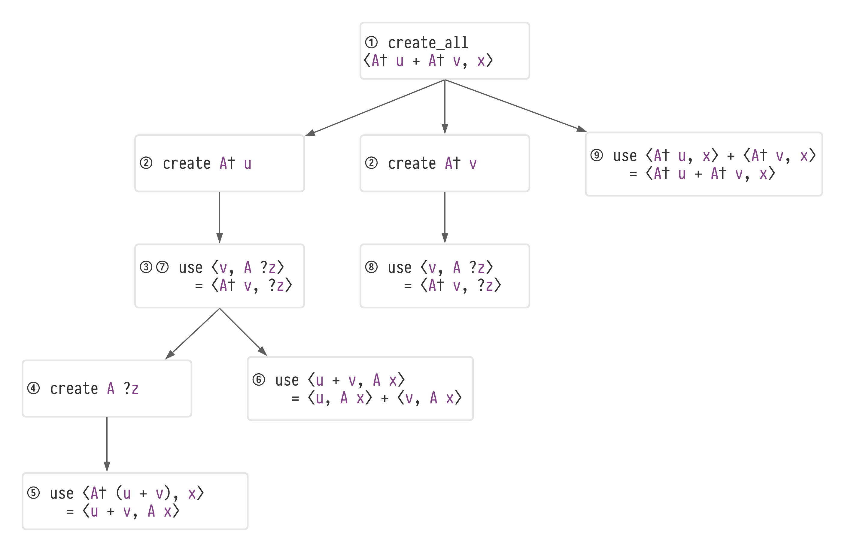
The tree in Figure 4.5 represents what the algorithm does with the additivity-of-adjoint problem (4.3). It starts with the subtask create_all ⟨𝐴† 𝑢 + 𝐴† v, x⟩ at ①. Since it cannot achieve that in one application of an available rule, it creates a set of subtasks and then chooses the one that is most promising: later in Section 4.3, I will explain how it generates and evaluates possible subtasks. In this case the most promising subtask is create 𝐴† 𝑢, so it selects that in ② and identifies a rewrite rule - the definition of adjoint: ∀ 𝑤 𝑧, ⟨𝐴† 𝑤, 𝑧⟩ = ⟨𝑤, 𝐴 𝑧⟩ - that can achieve it; adding use ⟨𝑢, 𝐴 ?𝑧⟩ = ⟨𝐴† 𝑢, ?𝑧⟩ to the tree at ③. The ?𝑧 that appears at ③ in Figure 4.5 is a metavariableThat is, a placeholder for an expression to be chosen later. See Section 2.4 for background information on metavariables. that will in due course be assigned to 𝑥. Now the process repeats on ③, a set of subtasks are again created for the lhs of ⟨𝑢, 𝐴 ?𝑧⟩ = ⟨𝐴† 𝑢, ?𝑧⟩ and the subtask create 𝐴 ?𝑧 is selected (④). Now, there does exist a rewrite rule that will achieve create 𝐴 ?𝑧: ⟨𝐴† (𝑢 + 𝑣), 𝑥⟩ = ⟨𝑢 + 𝑣, 𝐴 𝑥⟩, so this is applied and now the algorithm iterates back up the subtask tree, testing whether the new expression ⟨𝑢 + 𝑣, 𝐴 𝑥⟩ achieves any of the subtasks and whether any new rewrite rules can be used to achieve them.

In the next section, I will provide the design of an algorithm that behaves according to these motivating principles.

4.3. Design of the algorithm

The subtasks algorithm may be constructed as a search over a directed graph S.

The subtask algorithm's state 𝑠 : S has three components ⟨𝑡, 𝑓, 𝑐⟩:

a tree 𝑡𝑠 : Tree(Task) of tasks (as depicted in Figure 4.5)
a 'focussed' node 𝑓 : Address(𝑡𝑠) in the tree𝑡𝑠 and 𝑓 are implemented as a zipper [Hue97]. Zippers are described in Appendix A..
an expression 𝑐 : Expr called the current expression (CE) which represents the current left-hand-side of the equality chain. The subtasks algorithm provides the edges between states through sound manipulations of the tree and current expression. Each task in the tree corresponds to a predicate or potential rule application that could be used to solve an equality problem.

Given an equational reasoning problem Γ ⊢ 𝑙 = 𝑟, the initial state 𝑠₀ : S consists of a tree with a single root node CreateAll 𝑟 and a CE 𝑙. We reach a goal state when the current expression 𝑐 is definitionally equalThat is, the two expressions are equal by reflexivity. to 𝑟.

The first thing to note is that if we project 𝑠 : S to the current expression 𝑐, then we can recover the original equational rewriting problem E by taking the edges to be all possible rewrites between terms. One problem with searching this space is that the number of edges leaving an expression can be infiniteFor example, the rewrite rule ∀ 𝑎 𝑏, 𝑎 = 𝑎 - 𝑏 + 𝑏 can be applied to any expression with any expression being substituted for 𝑏. The typical way that this problem is avoided is to first ground all available rewrite rules by replacing all free variables with relevant expressions. The subtasks algorithm does not do this, because this is not a step that humans perform when solving simple equality problems. Even after grounding, the combinatorial explosion of possible expressions makes E a difficult graph to search without good heuristics. The subtasks algorithm makes use of the subtasks tree 𝑡 to guide the search in E in a manner that is intended to match the process outlined in List 4.4 and Figure 4.5.

A task 𝑡 : Task implements the following three methods:

refine : Task → (List Task) creates a list of subtasks for a given task. For example, a task create (𝑥 + 𝑦) would refine to subtasks create 𝑥, create 𝑦. The refinement may also depend on the current state 𝑠 of the tree and CE. The word 'refinement' was chosen to reflect its use in the classic paper by Kambhampati [KKY95[KKY95]Kambhampati, Subbarao; Knoblock, Craig A; Yang, QiangPlanning as refinement search: A unified framework for evaluating design tradeoffs in partial-order planning (1995)Artificial Intelligencehttps://doi.org/10.1016/0004-3702(94)00076-D]; a refinement is the process of splitting a set of candidate solutions that may be easier to check separately.
test : Task → Expr → Bool which returns true when the given task 𝑡 : Task is achieved for the given current expression 𝑒 : Expr. For example, if the current expression is 4 + 𝑥, then create 𝑥 is achieved. Hence, each task may be viewed as a predicate over expressions.
Optionally, execute : Task → Option Rewrite which returns a Rewrite object representing a rewrite rule from the current expression 𝑐ᵢ to some new expression 𝑐ᵢ₊₁ (in the context Γ) by providing a proof 𝑐ᵢ = 𝑐ᵢ₊₁ that is checked by the prover's kernel. Tasks with execute functions are called strategies. In this case, test must return true when execute can be applied successfully, making test a precondition predicate for execute. As an example, the use (𝑥 = 𝑦) task performs the rewrite 𝑥 = 𝑦 whenever the current expression contains an instance of 𝑥.

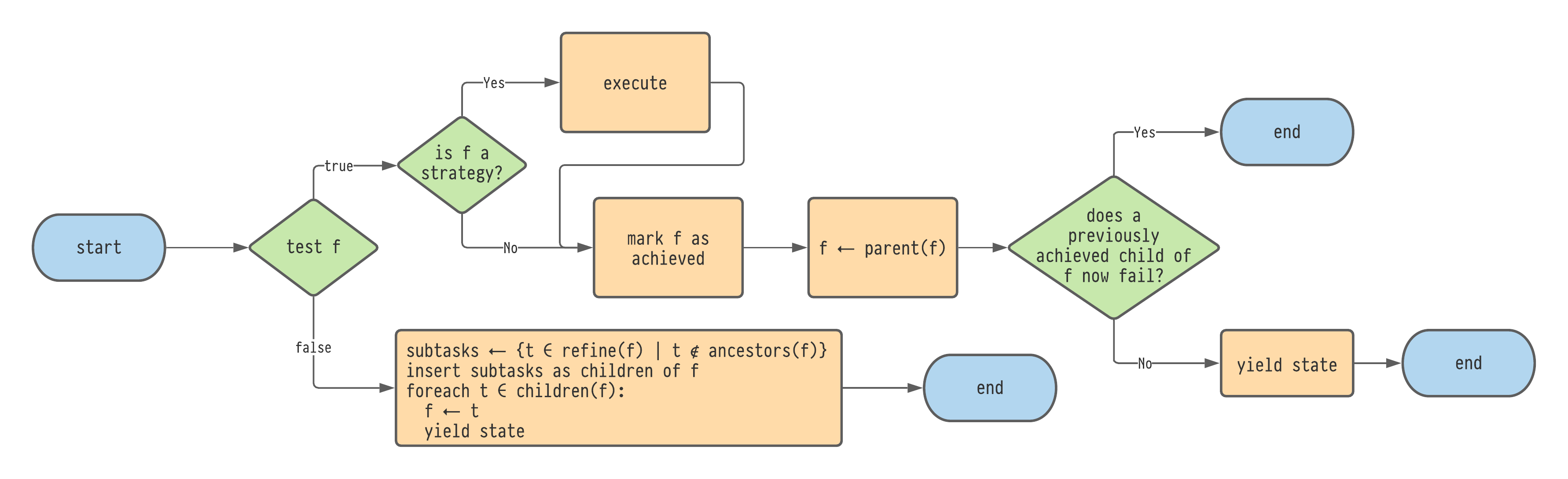
This design enables the system to be modular, where different sets of tasks and strategies can be included. Specific examples of tasks and strategies used by the algorithm are given in {#the-main-subtasks}. Given a state 𝑠 : S, the edges leading from 𝑠 are generated using the flowchart shown in Figure 4.6.

Let 𝑓 be the focussed subtask for 𝑠. In the case that test(𝑓) is true the algorithm 'ascends' the task tree. In this branch, 𝑓 is tagged as 'achieved' and the new focussed task is set as parent of 𝑓. Then, it is checked whether any siblings of 𝑓 that were marked as achieved are no longer achieved (that is, there is a sibling task 𝑡 tagged as achieved but test(𝑡) is now false). The intuition behind this check on previously achieved subtasks is that once a sibling task is achieved, it should not be undone by a later step because the assumption is that all of the child subtasks are needed before the parent task can be achieved.

In the case that test(𝑓) is false, meanwhile, the algorithm 'explores' the task tree by finding new child subtasks for 𝑓. To do this, refine(𝑓) is called to produce a set of candidate subtasks for 𝑓. For each 𝑡 ∈ refine(𝑓), 𝑡 is inserted as a child of 𝑓 provided that test(𝑡) is false and 𝑡 does not appear as an ancestor of 𝑓. Duplicate children are removed. Finally, for each subtask 𝑡, a new state is yielded with the focus now set to 𝑡. Hence 𝑠's outdegreeThe outdegree of a vertex 𝑣 in a directed graph is the number of edges leaving 𝑣. in the graph will be the number of children that 𝑓 has after refining.

**Figure 4.6**
Flowchart for generating edges for a starting state `𝑠 : S`. Here, each call to `yield state` will produce another edge leading from `𝑠` to the new state.

Now that the state space S, the initial state 𝑠₀, the goal states and the edges on S are defined, we can perform a search on this graph with the help of a heuristic function h : S → [0, ∞] to be discussed in Section 4.3.2. The subtasks algorithm uses greedy best-first search with backtracking points. However, other graph-search algorithms such as A⋆ or hill-climbing may be used.

4.3.1. The defined subtasks

In this section I will provide a list of the subtasks that are implemented in the system and some justification for their design.

4.3.1.1. `create_all 𝑒`

The create_all : Expr → Task task is the root task of the subtask tree.

Refine: returns a list of create 𝑏 subtasks where each 𝑏 is a minimal subterm of 𝑒 not present in the current expression.
Test: true whenever the current expression is 𝑒. If this task is achieved then the subtasks algorithm has succeeded in finding an equality chain.
Execute: none.

The motivation behind the refinement rule is that since 𝑏 appears in 𝑒 but not in the current expression, then it must necessarily arise as a result of applying a rewrite rule. Rather than include every subterm of 𝑒 with this property, we need only include the minimal subterms with this property since if 𝑏 ⊂ 𝑏', then test(create 𝑏) ⇐ test(create 𝑏'). In the running example (4.3), the subtasks of create_all ⟨𝐴† 𝑢 + 𝐴† 𝑣, 𝑥⟩ are create (𝐴† 𝑢) and create (𝐴† 𝑣).

4.3.1.2. `create 𝑒`

The create task is achieved if the current expression contains 𝑒.

Refine: returns a list use (𝑎 = 𝑏) subtasks where 𝑒 overlaps with 𝑏 (see further discussion below). It can also return reduce_distance subtasks in some circumstances.
Test: true whenever the current expression is 𝑒.
Execute: none.

Given a rewrite rule 𝑟 : ∀ (..𝑥𝑠), 𝑎 = 𝑏, say that an expression 𝑒 overlaps with the right hand side of 𝑟 when there exists a most-general substitution σ on 𝑟's variables 𝑥𝑠 such that

𝑒 appears in σ(𝑏);
𝑒 does not appear in σ(𝑎);
𝑒 does not appear in σ. This last condition ensures that the expression comes about as a result of the term-structure of the rule 𝑟 itself rather than as a result of a substitution. The process of determining these rules is made efficient by storing the available rewrite rules in a term indexed datastructure [SRV01[SRV01]Sekar, R; Ramakrishnan, I.V.; Voronkov, AndreiTerm Indexing (2001)Handbook of automated reasoninghttps://dl.acm.org/doi/abs/10.5555/778522.778535].

Additionally, as mentioned, create 𝑒 can sometimes refine to yield a reduce_distance subtask. The condition for this depends on the distance between two subterms in a parent expression 𝑐 : Expr, which is defined as the number of edges between the roots of the subterms -- viewing 𝑐's expression tree as a graph. If two local variables 𝑥, 𝑦 are present exactly once in both the current expression and 𝑒, and the distance between them is greater in the current expression, then reduce_distance 𝑥 𝑦 is included as a subtask.

In order to handle cases where multiple copies of 𝑒 are required, create has an optional count argument that may be used to request an nth copy of 𝑒.

4.3.1.3. `use (𝑎 = 𝑏)`

This is the simplest strategy. It simply represents the subtask of using the given rewrite rule.

Refine: Returns a list of create 𝑒 subtasks where each 𝑒 is a minimal subterm of 𝑎 not present in the current expression. This is the same refinement rule that is used to create subtasks of the create_all task.
Test: True whenever the rule 𝑎 = 𝑏 can be applied to the current expression.
Execute: Apply 𝑎 = 𝑏 to the current expression. In the event that it fails (for example if the rule application causes an invalid assignment of a metavariable) then the strategy fails.

4.3.1.4. `reduce_distance (𝑥, 𝑦)`

reduce_distance is an example of a greedy, brute-force strategy. It will perform any rewrite rule that moves the given variables closer together and then terminate.

Refine: returns the empty list. That is, there are no subtasks available.
Test: True whenever there is only one instance of 𝑥 and 𝑦 in the current expression and there exists a rewrite rule that will move 𝑥 closer to 𝑦.
Execute: repeatedly applies rewrite rules greedily moving 𝑥 and 𝑦 closer together, terminating when they can move no further together.

4.3.2. Heuristics

In this section I present the heuristic function developed for the subtasks algorithm. The ideas behind this function are derived from introspection on equational reasoning and some degree of trial and error on a set of equality problems.

There are two heuristic functions that are used within the system, an individual strategy heuristic and an 'overall-score' heuristic that evaluates sets of child strategies for a particular task. Overall-score is used on tasks which are not strategies by performing a lookahead of the child strategies of the task. The child strategies 𝑆₁, 𝑆₂ ⋯ are then scored individually through a scoring system, scoring higher if they:

achieve a task higher in the task tree;
achieve a task on a different branch of the task tree;
have a high degree of term overlap with the current expression. This is measured using symbol counting and finding largest common subterms;
use local variables and hypotheses;
can be achieved in one rewrite step from the current expression.

The intuition behind all of these is to give higher scores to strategies that are salient in some way, either by containing subterms that are present in the current expression or because other subtasks are achieved.

From these individual scores, the score for the parent task of 𝑆₁, 𝑆₂ ... is computed as follows: If there is only one strategy then it scores 10. If there are multiple strategies, it discards any scoring less than -5. If there are positive-scoring strategies then all negative-scoring strategies are discarded. The overall score is then set to be 5 minus the number of strategies in the list. The intention of this procedure is that smaller sets of strategies should be preferred, even if their scores are bad because it limits choice in what to do next.

The underlying idea behind the overall-scoring heuristic is that often the first sensible strategy found is enough of a signpost to solve simple problems. That is, once one has found one plausible strategy of solving a simple problem it is often fruitful to stop looking for other strategies which achieve the same thing and to get on with finding a way of performing the new strategy.

4.3.3. Properties of the algorithm

The substasks algorithm is sound provided sound rewrite rules are produced by the function execute : Task → Option Rewrite. That is, given an equation to solve Γ ⊢ 𝑙 = 𝑟 and given a path 𝑠₀ ↝ 𝑠₁ ↝ ... ↝ 𝑠ₙ in S where 𝑠₀ is the initial state defined in By forgetting the subtask tree, a solution path in S can be projected to a solution path in E, the equational rewriting graph. This projected path is exactly a proof of 𝑙 = 𝑟; it will be composed of a sequence 𝑙 ≡ 𝑐₀ = 𝑐₁ = ... = 𝑐ₙ ≡ 𝑟 where 𝑐ᵢ is the current expression of 𝑠ᵢ. Each equality in the chain holds either by the assumption of the proofs returned from execute being sound or by the fact that the current expression doesn't change between steps otherwise.

The next question to ask is whether S is complete with respect to E. That is, does S contain a path to the solution whenever E contains one? The answer to this depends on the output of refine. If refine always returns an empty list of subtasks then S is not complete, because no subtasks will ever be executed. The set of subtasks provided in Section 4.3.1 are not complete. For example the problem 1 - 1 = 𝑥 + - 𝑥 will not solve without additional subtasks since the smallest non-present subterm is 𝑥, so create 𝑥 is added which then does not refine further using the procedure in Section 4.3.1. In Section 4.6 I will discuss some methods to address this.

There has been a substantial amount of research on the automation of solving equality chain problems over the last decade. The approach of the subtasks algorithm is to combine these rewriting techniques with a hierarchical search. In this section I compare subtasks which with this related work.

4.4.1. Term Rewriting

One way to find equality proofs is to perform a graph search using a heuristic. This is the approach of the rewrite-search algorithm by Hoek and Morrison [HM19[HM19]Hoek, Keeley; Morrison, Scottlean-rewrite-search GitHub repository (2019)https://github.com/semorrison/lean-rewrite-search], which uses the heuristic of string edit-distance between the strings' two pretty-printed expressions. The rewrite-search algorithm does capture some human-like properties in the heuristic, since the pretty printed expressions are intended for human consumption. The subtasks algorithm is different from rewrite-search in that the search is guided according to achieving sequences of tasks. Since both subtasks and rewrite-search are written in Lean, some future work could be to investigate a combination of both systems.

A term rewriting system (TRS) 𝑅 is a set of oriented rewrite rules. There are many techniques available for turning a set of rewrite rules in to procedures that check whether two terms are equal. One technique is completion, where 𝑅 is converted into an equivalent TRS 𝑅' that is convergent. This means that any two expressions 𝑎, 𝑏 are equal under 𝑅 if and only if repeated application of rules in 𝑅' to 𝑎 and 𝑏 will produce the same expression. Finding equivalent convergent systems, if not by hand, is usually done by finding decreasing orderings on terms and using Knuth-Bendix completion [KB70[KB70]Knuth, Donald E; Bendix, Peter BSimple word problems in universal algebras (1970)Computational Problems in Abstract Algebrahttps://www.cs.tufts.edu/~nr/cs257/archive/don-knuth/knuth-bendix.pdf]. When such a system exists, automated rewriting systems can use these techniques to quickly find proofs, but the proofs are often overly long and needlessly expand terms.

Another method is rewrite tables, where a lookup table of representatives for terms is stored in a way that allows for two terms to be matched through a series of lookups.

Both completion and rewrite tables can be considered machine-oriented because they rely on large datastructures and systematic applications of rewrite rules. Such methods are certainly highly useful, but they can hardly be said to capture the process by which humans reason.

Finally, there are many normalisation and decision procedures for particular domains, for example on rings [GM05[GM05]Grégoire, Benjamin; Mahboubi, AssiaProving equalities in a commutative ring done right in Coq (2005)International Conference on Theorem Proving in Higher Order Logicshttp://cs.ru.nl/~freek/courses/tt-2014/read/10.1.1.61.3041.pdf]. Domain specific procedures do not satisfy the criterion of generality given in Section 4.1.

4.4.2. Proof Planning

Background information on proof planning is covered in Section 2.6.2.

The subtasks algorithm employs a structure that is similar to a hierarchical task network (HTN) [Sac74[Sac74]Sacerdoti, Earl DPlanning in a hierarchy of abstraction spaces (1974)Artificial intelligencehttps://doi.org/10.1016/0004-3702(74)90026-5, Tat77[Tat77]Tate, AustinGenerating project networks (1977)Proceedings of the 5th International Joint Conference on Artificial Intelligence.https://dl.acm.org/doi/abs/10.5555/1622943.1623021, MS99[MS99]Melis, Erica; Siekmann, JörgKnowledge-based proof planning (1999)Artificial Intelligencehttps://doi.org/10.1016/S0004-3702(99)00076-4]. The general idea of a hierarchical task network is to break a given abstract task (e.g., "exit the room") in to a sequence of subtasks ("find a door" then "go to door" then "walk through the door") which may themselves be recursively divided into subtasks ("walk through the door" may have a subtask of "open the door" which may in turn have "grasp doorhandle" until bottoming out with a ground actuation such as "move index finger 10°"). This approach has found use for example in the ICARUS robotics architecture [CL18[CL18]Choi, Dongkyu; Langley, PatEvolution of the ICARUS cognitive architecture (2018)Cognitive Systems Researchhttps://doi.org/10.1016/j.cogsys.2017.05.005, LCT08[LCT08]Langley, Pat; Choi, Dongkyu; Trivedi, NishantIcarus user’s manual (2008)http://www.isle.org/~langley/papers/manual.pdf]. HTNs have also found use in proof planning [MS99[MS99]Melis, Erica; Siekmann, JörgKnowledge-based proof planning (1999)Artificial Intelligencehttps://doi.org/10.1016/S0004-3702(99)00076-4].

The main difference between the approach used in the subtasks algorithm and proof planning and hierarchical task networks is that the subtasks algorithm is greedier: the subtasks algorithm generates enough of a plan to have little doubt what the first rewrite rule in the sequence should be, and no more. I believe that this reflects how humans reason for solving simple problems: favouring just enough planning to decide on a good first step, and then planning further only once the step is completed and new information is revealed.

A difference between HTNs and subtasks is that the chains of subtasks do not necessarily reach a ground subtask (for subtasks this is a rewrite step that can be performed immediately). This means that the subtasks algorithm needs to use heuristics to determine whether it is appropriate to explore a subtask tree or not instead of relying on the task hierarchy eventually terminating with ground tasks. The subtasks algorithm also inherits all of the problems found in hierarchical planning: the main one being finding heuristics for determining whether a subtask should be abandoned or refined further. The heuristics given in Section 4.3.2 help with this but there are plenty more ideas from the hierarchical task planning literature that could be incorporated also. Of particular interest for me are the applications of hierarchical techniques from the field of reinforcement learningA good introductory text to modern reinforcement learning is Reinforcement Learning; An Introduction by Sutton and Barto [SB18b]. Readers wishing to learn more about hierarchical reinforcement learning may find this survey article by Flet-Berliac to be a good jumping-off point [Fle19].[SB18b]Sutton, Richard S; Barto, Andrew GReinforcement learning: An introduction (2018)publisher MIT presshttp://incompleteideas.net/book/the-book-2nd.html[Fle19]Flet-Berliac, YannisThe Promise of Hierarchical Reinforcement Learning (2019)The Gradienthttps://thegradient.pub/the-promise-of-hierarchical-reinforcement-learning.

4.5. Evaluation

The ultimate motivation behind the subtasks algorithm is to make an algorithm that behaves as a human mathematician would. I do not wish to claim that I have fully achieved this, but we can evaluate the algorithm with respect to the general goals that were given in Chapter 1.

Scope: can it solve simple equations?
Generality: does it avoid techniques specific to a particular area of mathematics?
Reduced search space: does the algorithm avoid search when finding proofs that humans can find easily without search?
Straightforwardness of proofs: for easy problems, does it give a proof that an experienced human mathematician might give?

The method of evaluation is to use the algorithm implemented as a tactic in Lean on a library of thirty or so example problems. This is not large enough for a substantial quantitative comparison with existing methods, but we can still investigate some properties of the algorithm. The source code also contains many examples which are outside the abilities of the current implementation of the algorithm. Some ways to address these issues are discussed in Section 4.6.

Table 4.7 gives some selected examples. These are all problems that the algorithm can solve with no backtracking.

Table 4.7

subtask's performance on some example problems. Steps gives the number of rewrite steps in the final proof. Location gives the file and declaration name of the example in the source code.

Problem	Steps	Location
`𝑕 : α` `𝑙 𝑠 : List α` `rev(𝑙 ++ 𝑠) = rev(𝑠) ++ rev(𝑙)` `∀ 𝑎, rev(𝑎 :: 𝑙) = rev(𝑙) ++ [𝑎]` `rev(𝑕 :: 𝑙 ++ 𝑠) = rev(𝑠) ++ rev(𝑕 :: 𝑙)`	5	`datatypes.lean/rev_app_rev`
`A : Monoid` `𝑎 : A` `𝑚 𝑛 : ℕ` `𝑎 ^ (𝑚 + 𝑛) = 𝑎 ^ 𝑚 * 𝑎 ^ 𝑚` `𝑎 ^ (succ(𝑚) + 𝑛) = 𝑎 ^ succ(𝑚) * 𝑎 ^ 𝑛`	8	`groups.lean/my_pow_add`
`R : Ring` `𝑎 𝑏 𝑐 𝑑 𝑒 𝑓 : R` `𝑎 * 𝑑 = 𝑐 * 𝑑` `𝑐 * 𝑓 = 𝑒 * 𝑏` `𝑑 * (𝑎 * 𝑓) = 𝑑 * (𝑒 * 𝑏)`	9	`rat.lean`
`R : Ring` `𝑎 𝑏 : R` `(𝑎 + 𝑏) * (𝑎 + 𝑏) = 𝑎 * 𝑎 + 2 * (𝑎 * 𝑏) + 𝑏 * 𝑏`	7	`rings.lean/sumsq_with_equate`
`𝐵 𝐶 𝑋 : set` `𝑋 \ (𝐵 ∪ 𝐶) = (𝑋 \ 𝐵) \ 𝐶`	4	`sets.lean/example_4`

From this Table 4.7 we can see that the algorithm solves problems from several different domains. I did not encode any decision procedures for monoids or rings. In fact I did not even include reasoning under associativity and commutativity, although I am not in principle against extending the algorithm to do this. The input to the algorithm is a list of over 100 axioms and equations for sets, rings, groups and vector spaces which can be found in the file equate.lean in the source codehttps://github.com/EdAyers/lean-subtask. Thus, the algorithm exhibits considerable generality.

All of the solutions to the above examples are found without backtracking, which adds support to the claim that the subtasks algorithm requires less search. There are, however, other examples in the source where backtracking occurs.

The final criterion is that the proofs are more straightforward than those produced by machine-oriented special purpose tactics. This is a somewhat subjective measure but there are some proxies that indicate that subtasks can be used to generate simpler proofs.

To illustrate this point, consider the problem of proving (𝑥 + 𝑦)² + (𝑥 + 𝑧)² = (𝑧 + 𝑥)² + (𝑦 + 𝑥)² within ring theory. I choose this example because it is easy for a human to spot how to do it with three uses of commutativity, but it is easy for a program to be led astray by expanding the squares. subtask proves this equality with 3 uses of commutativity and with no backtracking or expansion of the squares. This is an example where domain specific tactics do worse than subtask, the ring tactic for reasoning on problems in commutative rings will produce a proof by expanding out the squares. The built-in tactics ac_refl and blast in Lean which reason under associativity and commutativity both use commutativity 5 times. If one is simply interested in verification, then such a result is perfectly acceptable. However, I am primarily interested in modelling how humans would solve such an equality, so I want the subtasks algorithm not to perform unnecessary steps such as this.

It is difficult to fairly compare the speed of subtask in the current implementation because it is compiled to Lean bytecode which is much slower than native built-in tactics that are written in C++. However it is worth noting that, even with this handicap, subtask takes 1900ms to find the above proof whereas ac_refl and blast take 600ms and 900ms respectively.

There are still proofs generated by subtask that are not straightforward. For example, the lemma (𝑥 * 𝑧) * (𝑧⁻¹ * 𝑦) = 𝑥 * 𝑦 in group theory is proved by subtask with a superfluous use of the rule e = 𝑥 * 𝑥⁻¹.

4.6. Conclusions and Further Work

In this chapter, I introduced a new, task-based approach to finding equalities in proofs and provided a demonstration of the approach by building the subtask tactic in Lean. I show that the approach can solve simple equality proofs with very little search. I hope that this work will renew interest in proof planning and spark interest in human-oriented reasoning for at least some classes of problems.

In future work, I wish to add more subtasks and better heuristics for scoring them. The framework I outlined here allows for easy experimentation with such different sets of heuristics and subtasks. In this way, I also wish to make the subtask framework extensible by users, so that they may add their own custom subtasks and scoring functions.

Another possible extension of the subtasks algorithm is to inequality chains. The subtasks algorithm was designed with an extension to inequalities in mind, however there are some practical difficulties with implementing it. The main difficulty with inequality proofs is that congruence must be replaced by appropriate monoticity lemmas. For example, 'rewriting' 𝑥 + 2 ≤ 𝑦 + 2 using 𝑥 < 𝑦 requires the monotonicity lemma ∀ 𝑥 𝑦 𝑧, 𝑥 ≤ 𝑦 → 𝑥 + 𝑧 ≤ 𝑦 + 𝑧. Many of these monotonicity lemmas have additional goals that need to be discharged such as 𝑥 > 0 in 𝑦 ≤ 𝑧 → 𝑥 * 𝑦 ≤ 𝑥 * 𝑧, and so the subtasks algorithm will need to be better integrated with a prover before it can tackle inequalities.

There are times when the algorithm fails and needs guidance from the user. I wish to study further how the subtask paradigm might be used to enable more human-friendly interactivity than is currently possible. For example, in real mathematical textbooks, if an equality step is not obvious, a relevant lemma will be mentioned. Similarly, I wish to investigate ways of passing 'hint' subtasks to the tactic. For example, when proving 𝑥 * 𝑦 = (𝑥 * 𝑧) * (𝑧⁻¹ * 𝑦), the algorithm will typically get stuck (although it can solve the flipped problem), because there are too many ways of creating 𝑧. However, the user - upon seeing subtask get stuck - could steer the algorithm with a suggested subtask such as create (𝑥 * (𝑧 * 𝑧⁻¹)).

Using subtasks should help to give better explanations to the user. The idea of the subtasks algorithm is that the first set of strategies in the tree roughly corresponds to the high-level actions that a human would first consider when trying to solve the problem. Thus, the algorithm could use the subtask hierarchy to determine when no further explanation is needed and thereby generate abbreviated proofs of a kind that might be found in mathematical textbooks.

Another potential area to explore is to perform an evaluation survey where students are asked to determine whether an equality proof was generated by the software or a machine.

Bibliography for this chapter

[AGJ19]Ayers, E. W.; Gowers, W. T.; Jamnik, MatejaA human-oriented term rewriting system (2019)KI 2019: Advances in Artificial Intelligence - 42nd German Conference on AIvolume 11793pages 76--86editors Benzmüller, Christoph; Stuckenschmidt, Heinerorganization Springerpublisher Springerdoi 10.1007/978-3-030-30179-8_6https://www.repository.cam.ac.uk/bitstream/handle/1810/298199/main.pdf?sequence=1
[BN98]Baader, Franz; Nipkow, TobiasTerm rewriting and all that (1998)publisher Cambridge University Pressisbn 978-0-521-45520-6https://doi.org/10.1017/CBO9781139172752
[CL18]Choi, Dongkyu; Langley, PatEvolution of the ICARUS cognitive architecture (2018)Cognitive Systems Researchvolume 48pages 25--38publisher Elsevierdoi 10.1016/j.cogsys.2017.05.005https://doi.org/10.1016/j.cogsys.2017.05.005
[Fle19]Flet-Berliac, YannisThe Promise of Hierarchical Reinforcement Learning (2019)The Gradienthttps://thegradient.pub/the-promise-of-hierarchical-reinforcement-learning
[GM05]Grégoire, Benjamin; Mahboubi, AssiaProving equalities in a commutative ring done right in Coq (2005)International Conference on Theorem Proving in Higher Order Logicsvolume 3603pages 98--113editors Hurd, Joe; Melham, Thomas F.organization Springerdoi 10.1007/11541868_7http://cs.ru.nl/~freek/courses/tt-2014/read/10.1.1.61.3041.pdf
[HM19]Hoek, Keeley; Morrison, Scottlean-rewrite-search GitHub repository (2019)https://github.com/semorrison/lean-rewrite-search
[Hue97]Huet, GérardFunctional Pearl: The Zipper (1997)Journal of functional programmingvolume 7number 5pages 549--554publisher Cambridge University Presshttp://www.st.cs.uni-sb.de/edu/seminare/2005/advanced-fp/docs/huet-zipper.pdf
[KB70]Knuth, Donald E; Bendix, Peter BSimple word problems in universal algebras (1970)Computational Problems in Abstract Algebrapages 263-297editor Leech, Johnpublisher Pergamondoi https://doi.org/10.1016/B978-0-08-012975-4.50028-Xisbn 978-0-08-012975-4https://www.cs.tufts.edu/~nr/cs257/archive/don-knuth/knuth-bendix.pdf
[KKY95]Kambhampati, Subbarao; Knoblock, Craig A; Yang, QiangPlanning as refinement search: A unified framework for evaluating design tradeoffs in partial-order planning (1995)Artificial Intelligencevolume 76number 1pages 167--238doi 10.1016/0004-3702(94)00076-Dhttps://doi.org/10.1016/0004-3702(94)00076-D
[LCT08]Langley, Pat; Choi, Dongkyu; Trivedi, NishantIcarus user’s manual (2008)institution Institute for the Study of Learning and Expertisehttp://www.isle.org/~langley/papers/manual.pdf
[MKA+15]de Moura, Leonardo; Kong, Soonho; Avigad, Jeremy; Van Doorn, Floris; von Raumer, JakobThe Lean theorem prover (system description) (2015)International Conference on Automated Deductionvolume 9195pages 378--388editors Felty, Amy P.; Middeldorp, Aartorganization Springerdoi 10.1007/978-3-319-21401-6_26https://doi.org/10.1007/978-3-319-21401-6_26
[MS99]Melis, Erica; Siekmann, JörgKnowledge-based proof planning (1999)Artificial Intelligencevolume 115number 1pages 65--105editor Bobrow, Daniel G.publisher Elsevierdoi 10.1016/S0004-3702(99)00076-4https://doi.org/10.1016/S0004-3702(99)00076-4
[Sac74]Sacerdoti, Earl DPlanning in a hierarchy of abstraction spaces (1974)Artificial intelligencevolume 5number 2pages 115--135publisher Elsevierdoi 10.1016/0004-3702(74)90026-5https://doi.org/10.1016/0004-3702(74)90026-5
[SB18b]Sutton, Richard S; Barto, Andrew GReinforcement learning: An introduction (2018)publisher MIT presshttp://incompleteideas.net/book/the-book-2nd.html
[SRV01]Sekar, R; Ramakrishnan, I.V.; Voronkov, AndreiTerm Indexing (2001)Handbook of automated reasoningvolume 2pages 1855--1900editors Robinson, Alan; Voronkov, Andreipublisher Elsevierhttps://dl.acm.org/doi/abs/10.5555/778522.778535
[Tat77]Tate, AustinGenerating project networks (1977)Proceedings of the 5th International Joint Conference on Artificial Intelligence.pages 888--893editor Reddy, Rajorganization Morgan Kaufmann Publishers Inc.doi 10.5555/1622943.1623021https://dl.acm.org/doi/abs/10.5555/1622943.1623021