A Tool for Producing Verified, Explainable Proofs.
Edward William Ayers
Corpus Christi College
University of Cambridge
Submission Date: 2021-09-06
This thesis is submitted for the degree of Doctor of Philosophy.
This thesis is the result of my own work and includes nothing which is the outcome of work done in collaboration except as declared in the preface and specified in the text. It is not substantially the same as any work that has already been submitted before for any degree or other qualification except as declared in the preface and specified in the text. It does not exceed the prescribed word limit for the Mathematics Degree Committee.
Abstract
Mathematicians are reluctant to use interactive theorem provers. In this thesis I argue that this is because proof assistants don't emphasise explanations of proofs; and that in order to produce good explanations, the system must create proofs in a manner that mimics how humans would create proofs. My research goals are to determine what constitutes a human-like proof and to represent human-like reasoning within an interactive theorem prover to create formalised, understandable proofs. Another goal is to produce a framework to visualise the goal states of this system.
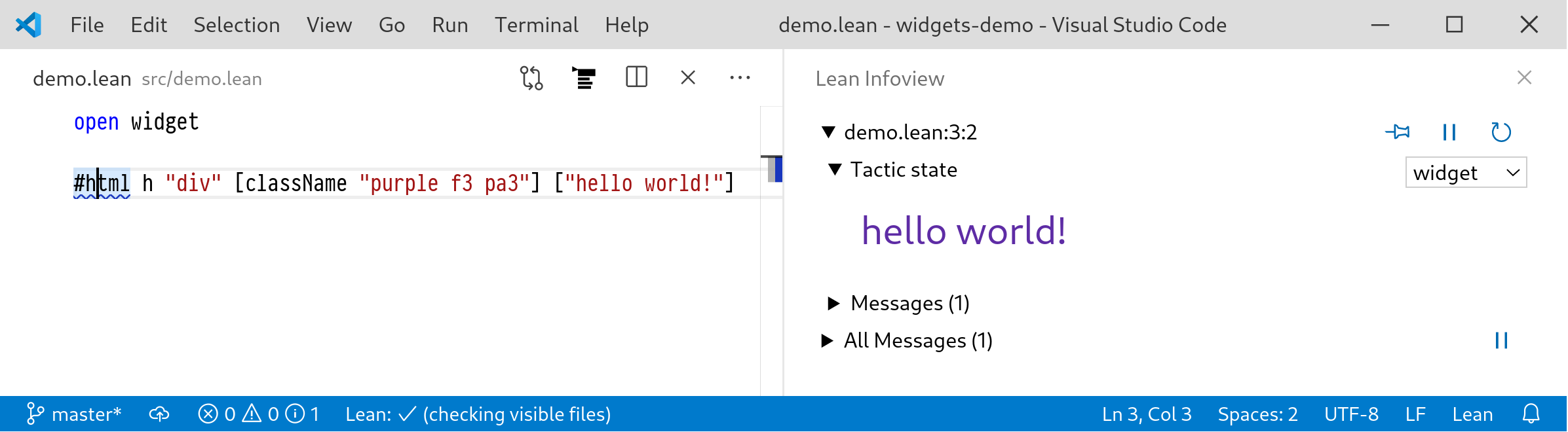
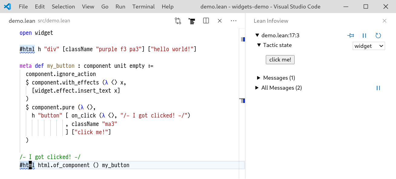
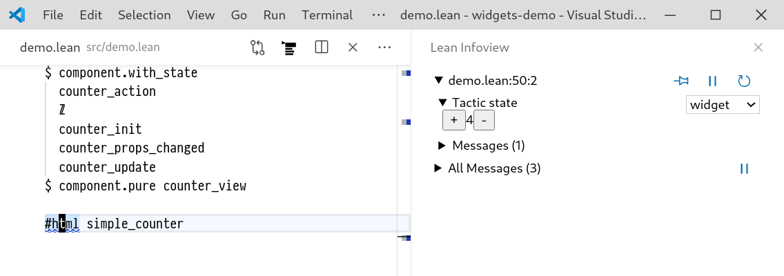
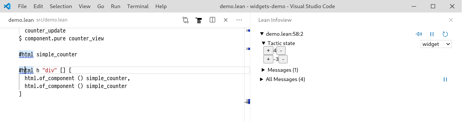
To demonstrate this, I present HumanProof: a piece of software built for the Lean 3 theorem prover. It is used for interactively creating proofs that resemble how human mathematicians reason. The system provides a visual, hierarchical representation of the goal and a system for suggesting available inference rules. The system produces output in the form of both natural language and formal proof terms which are checked by Lean's kernel. This is made possible with the use of a structured goal state system which interfaces with Lean's tactic system which is detailed in Chapter 3.
In Chapter 4, I present the subtasks automation planning subsystem, which is used to produce equality proofs in a human-like fashion. The basic strategy of the subtasks system is break a given equality problem in to a hierarchy of tasks and then maintain a stack of these tasks in order to determine the order in which to apply equational rewriting moves. This process produces equality chains for simple problems without having to resort to brute force or specialised procedures such as normalisation. This makes proofs more human-like by breaking the problem into a hierarchical set of tasks in the same way that a human would.
To produce the interface for this software, I also created the ProofWidgets system for Lean 3. This system is detailed in Chapter 5. The ProofWidgets system uses Lean's metaprogramming framework to allow users to write their own interactive, web-based user interfaces to display within the VSCode editor and in an online web-editor. The entire tactic state is available to the rendering engine, and hence expression structure and types of subexpressions can be explored interactively. The ProofWidgets system also allows the user interface to interactively edit the proof document, enabling a truly interactive modality for creating proofs; human-like or not.
In Chapter 6, the system is evaluated by asking real mathematicians about the output of the system, and what it means for a proof to be understandable to them. The user group study asks participants to rank and comment on proofs created by HumanProof alongside natural language and pure Lean proofs. The study finds that participants generally prefer the HumanProof format over the Lean format. The verbal responses collected during the study indicate that providing intuition and signposting are the most important properties of a proof that aid understanding.
My first contact with the ideas of formalised mathematics came from reading the anonymously authored QED Manifesto[Ano94[Ano94]AnonymousThe QED manifesto (1994)Automated Deduction--CADE(link)]In this thesis, shortened citation references will appear in the sidebar, a full bibliography with all reference details is provided at the end of the document. Some sidebar citations will be omitted if there is not enough space. which envisions a 'QED system' in which all mathematical knowledge is stored in a single, computer-verified repository.
This idea dizzied me: perhaps review of mathematics will amount to remarking on style and interest, with checking of proofs performed automatically from a machine readable document.
The general term that I will use for software that works towards this vision is proof assistant or Interactive Theorem Prover ITP. A proof assistant at its most general is a piece of software that allows users to create and verify mathematical proofs. In Section 2.1 I will provide more detail how proof assistants are generally constructed.
In 2007, Freek Wiedijk [Wie07[Wie07]Wiedijk, FreekThe QED manifesto revisited (2007)Studies in Logic, Grammar and Rhetoric(link)] pronounced the QED project to have "not been a success (yet)", citing not enough people working on formalised mathematics and the severe differences between formalised and 'real' mathematics, both at a syntactic level (formalised mathematics resembles source code) and at a foundational level (formalised mathematics is usually constructive and procedural as opposed to classical and declarative).
Similarly, Alan Bundy [Bun11[Bun11]Bundy, AlanAutomated theorem provers: a practical tool for the working mathematician? (2011)Annals of Mathematics and Artificial Intelligence(link)] notes that although mathematicians have readily adopted computational tools such as TEX[Knu86[Knu86]Knuth, Donald E.The TeXbook (1986)publisher Addison-Wesley] and computer algebra systemsA computer algebra system (CAS) is a tool for symbolic manipulation of formulae and expressions, without necessarily having a formalised proof that the manipulation is sound. Examples of CASes include Maple and Mathematica., computer aided proving has had very little impact on the workflow of a working mathematician. Bundy cites several reasons for this which will be discussed in Section 1.1.
Now, a decade later, the tide may be turning.
In 2021, proof assistants are pretty good. There are several well-supported large-scale systems such as Isabelle[Pau89], Coq[Coq], Lean[MKA+15], HOL Light[Har09], Agda[Nor08], Mizar[GKN15], PVS[SORS01] and many more. These systems are used to define and prove mathematical facts in a variety of logics (e.g. FOL, HOL, CIC, univalent foundations). These systems are bridged to powerful, automated reasoning systems (e.g. Vampire[RV02], Z3[MB08], E[SCV19] and Leo-III[SB18a]. Within these systems, many theorems big and small (4-colour theorem [Gon08], Feit-Thompson theorem [GAA+13], Kepler conjecture [HAB+17]) have been proved in a variety of fields, accompanied by large mathematical libraries (Isabelle's Archive of Formal Proofs, Lean's mathlib, Coq's Mathematical Components, Mizar's Formalized Mathematics) whose intersection with undergraduate and research level mathematics is steadily growingSee, for example, the rate of growth of the Lean 3 mathematical library https://leanprover-community.github.io/mathlib_stats.html..
However, in spite of these advances, we are still yet to see widespread adoption of ITP by mathematicians outside of some (growing) cliques of enthusiasts.
In this thesis I wish to address this problem through engaging with how mathematicians use and understand proofs to create new ways of interacting with formalised proof.
Let's first expand on the problem a little more and then use this to frame the research questions that I will tackle for the remainder of the thesis.
1.1. Mathematicians and proof assistants
Here I offer 3 possible explanations for why mathematicians have not adopted proof assistants.
Many have commented on these before: Bundy [Bun11] summarises the main challenges well.
1. Differing attitudes towards correctness and errors.
Mathematicians don't worry about mistakes in the same way as proof assistants doI will present some evidence for this in Section 2.5..
Mathematicians care deeply about correctness, but historically the dynamics determining whether a result is considered to be true are also driven by sociological mechanisms such as peer-review; informal correspondences; 'folk' lemmas and principles; reputation of authors; and so on [MUP79[MUP79]de Millo, Richard A; Upton, Richard J; Perlis, Alan JSocial processes and proofs of theorems and programs (1979)Communications of the ACM(link)].
A proxy for trustworthiness of a result is the number of other mathematicians that have scrutinized the work.
That is, if the proof is found on an undergraduate curriculum, you can predict with a high degree of confidence that any errors in the proof will be brought to the lecturer's attention.
In contrast, a standalone paper that has not yet been used for any subsequent work by others is typically treated with some degree of caution.
2. High cost.
Becoming proficient in an ITP system such as Isabelle or Coq can require a lot of time.
And then formalising an area of maths can take around ten times the amount of time required to write a corresponding paper or textbook on the topic.
This time quickly balloons if it is also necessary to write any underlying assumed knowledge of the topic (e.g., measure theory first requires real analysis).
This 'loss factor' of the space cost of developing a formalised proof over that of a natural language proof was first noted by de Bruijn in relation to his AUTOMATH prover [DeB80[DeB80]De Bruijn, Nicolaas GovertA survey of the project AUTOMATH (1980)To H.B.Curry: Essays on Combinatory Logic,Lambda Calculus and Formalism(link)]. De Bruijn estimates a factor of 20 for AUTOMATH, and Wiedijk later estimates this factor to be closer to three or four in Mizar[Wie00[Wie00]Wiedijk, FreekThe de Bruijn Factor (2000)http://www.cs.ru.nl/F.Wiedijk/factor/factor.pdf]. There are costs other than space too, the main one of concern here being the time to learn to use the tools and the amount of work required per proof.
3. Low reward.
What does a mathematician have to gain from formalising their research? In many cases, there is little to gain other than confirming something the researcher knew to be true anyway. The process of formalisation may bring to light 'bugs' in the work: perhaps there is a trivial case that wasn't accounted for or an assumption needs to be strengthened.
Sometimes the reward is high enough that there is a clear case for formalisation, particularly when the proof involves some computer-generated component.
This is exemplified by Hales' proof [Hal05[Hal05]Hales, Thomas CA proof of the Kepler conjecture (2005)Annals of mathematics(link)] and later formalised proof [HAB+17[HAB+17]Hales, Thomas C; Adams, Mark; Bauer, Gertrud; et al.A formal proof of the Kepler conjecture (2017)Forum of Mathematics, Pi(link)] of the Kepler conjecture. The original proof involved lengthy computer generated steps that were difficult for humans to check, and so Hales led the Flyspeck project to formalise it, taking 21 collaborators around a decade to complete.
Another celebrated example is Gonthier's formalisation of the computer-generated proof of the four-colour theorem [Gon08[Gon08]Gonthier, GeorgesFormal proof--the four-color theorem (2008)Notices of the AMS(link)].
Formalisation is also used regularly in formalising expensive hardware and safety-critical computer software (e.g., [KEH+09[KEH+09]Klein, Gerwin; Elphinstone, Kevin; Heiser, Gernot; et al.seL4: Formal verification of an OS kernel (2009)Proceedings of the ACM SIGOPS 22nd symposium on Operating systems principles(link), Pau98[Pau98]Paulson, Lawrence CThe inductive approach to verifying cryptographic protocols (1998)Journal of Computer Security(link)]).
The economics of the matter are such that the gains of using ITP are too low compared to the benefits for the majority of cases. Indeed, since mathematicians have a different attitude to correctness, there are sometimes no benefits to formalisation.
As ITP developers, we can improve the situation by either decreasing the learning cost or increasing the utility.
How can we make ITP easier to learn?
One way is to teach it in undergraduate mathematics curricula (not just computer science).
An example of such a course is Massot's Introduction aux mathématiques formalisées taught at the Université Paris Sud.
Another way is to improve the usability of the user interface for the proof assistant; I will consider this point in more detail in Chapter 5.
How can we increase the utility that mathematicians gain from using a proof assistant?
In this thesis I will argue that one way to help with these three issues is to put more emphasis on interactive theorem provers providing explanations rather than a mere guarantee of correctness.
We can see that explanations are important because mathematicians care about new proofs of old results that treat the problem in a new way.
Proofs from the Book[AZHE10[AZHE10]Aigner, Martin; Ziegler, Günter M; Hofmann, Karl H; et al.Proofs from the Book (2010)publisher Springer(link)] catalogues some particularly lovely examples of this.
Can computers also provide informal proofs with more emphasis on explanations?
Gowers [Gow10[Gow10]Gowers, W. T.Rough structure and classification (2010)Visions in Mathematics(link) §2] presents an imagined interaction between a mathematician and a proof assistant of the future.
Quotation 1.1
Excerpt from an imagined conversation between a mathematician and a computer from [Gow10 §2].
Mathematician. Is the following true? Let δ>0. Then for N sufficiently large, every set A⊆{1,2,...,N} of size at least δN contains a subset of the form {a,a+d,a+2d}?
Computer. Yes. If A is non-empty, choose a∈A and set d=0.
M. All right all right, but what if d is not allowed to be zero?
C. Have you tried induction on N, with some δ=δ(N) tending to zero?
M. That idea is no help at all. Give me some examples please.
C. The obvious greedy algorithm gives the set {1,2,4,5,10,11,13,14,28,29,31...}
An interesting feature of this conversation is that the status of the formal correctness of any of the statements conveyed by the computer is not mentioned.
Similar notions are brought to light in the work of Corneli et al.[CMM+17[CMM+17]Corneli, Joseph; Martin, Ursula; Murray-Rust, Dave; et al.Modelling the way mathematics is actually done (2017)Proceedings of the 5th ACM SIGPLAN International Workshop on Functional Art, Music, Modeling, and Design(link)] in their modelling of informal mathematical dialogues and exposition.
Why not have both explanatory and verified proofs? I suspect that if an ITP system is to be broadly adopted by mathematicians, it must concisely express theorems and their proofs in a way similar to that which a mathematician would communicate with fellow mathematicians.
This not only requires constructing human-readable explanations, but also a reimagining of how the user can interact with the prover.
In this thesis, I will focus on problems that are considered 'routine' for a mathematician.
That is, problems that a mathematician would typically do 'on autopilot' or by 'following their nose' For example, showing that (a+b)2=a2+2ab+b2 from the ring axioms..
I choose to focus on this class of problem because I believe it is an area where ITP could produce proofs that explain why they are true rather than merely provide a certificate of correctness. The typical workflow when faced with a problem like this is to either meticulously provide a low-level proof or apply automation such as Isabelle's auto, or an automation orchestration tool such as Isabelle's Sledgehammer [BN10[BN10]Böhme, Sascha; Nipkow, TobiasSledgehammer: judgement day (2010)International Joint Conference on Automated Reasoning(link)]. In the case of using an automation tacticBroadly, a tactic is a program for creating proofs. I will drill down on how this works in Chapter 2. like auto the tactic will either fail or succeed, leaving the user with little feedback on why the result is true.
There are some tools for producing intelligible proofs from formalised ones, for example, the creation of Isar [Wen99[Wen99]Wenzel, MarkusIsar - A Generic Interpretative Approach to Readable Formal Proof Documents (1999)Theorem Proving in Higher Order Logics(link)] proofs from Sledgehammer by Blanchette et al.[BBF+16[BBF+16]Blanchette, Jasmin Christian; Böhme, Sascha; Fleury, Mathias; et al.Semi-intelligible Isar proofs from machine-generated proofs (2016)Journal of Automated Reasoning(link)].
However, gaining an intuition for a proof will be easier if the proof is generated in a way that reflects how a human would solve the problem, and so translating a machine proof to a proof which a human will extract meaning from is an uphill battle.
1.1.1. Types of understandability
The primary motivation of the work in this thesis is to help make ITP systems more appealing to mathematicians.
The approach I chosen to take towards this is to research ways of making ITP systems more understandable.
There are many components of ITP that I consider with respect to understandability:
interaction: is the way in which the user interacts and creates a proof easy to understand?
system-output: is the final proof rendered to the user easy to understand?
underlying representations: is the way in which the proof is stored similar to the user's understanding of the proof?
automation: if a proof is generated automatically, is it possible for a user to follow it?
The different parts of my thesis will address different sets of these ways in which a proof assistant can be understandable.
With respect to the automation and underlying-representation aspects of understandability, we will see in Section 2.6 that there is some debate over whether prover automation needs to be easy to follow for a human or not (machine-like vs. human-like).
In this thesis I take a pragmatic stance that the understandability of automation and underlying-representation need not be human-like provided that the resulting interaction and output is understandable. However, as I investigate in Chapter 4, there may be ways of creating automation that are more conducive to creating understandable output and interaction.
1.2. Research questions
In the context of these facets of an understandable ITP system, there arise some key research questions that I seek to study.
Question 1. What constitutes a human-like, understandable proof?
Objectives:
Identify what 'human-like' and 'understandable' mean to different people.
Distinguish between human-like and machine-like proofs in the context of ITP.
Merge these strands to determine a working definition of human-like proof.
Question 2. How can human-like reasoning be represented within an interactive theorem prover to produce formalised, understandable proofs?
Objectives:
Form a calculus of representing goal states and inference steps that act at the abstraction layer that a human uses when solving proofs.
Create a system for producing natural language proofs from this calculus.
Evaluate the resulting system by performing a study on real mathematicians.
Question 3. How can this mode of human-like reasoning be presented to the user in an interactive, multimodal way?
Objectives:
Investigate new ways of interacting with proof objects.
Make it easier to create novel graphical user interfaces (GUIs) for interactive theorem provers.
Produce an interactive interface for a human-like reasoning system.
1.3. Contributions
This thesis presents a number of contributions towards the above research questions:
An abstract calculus for developing human-like proofs (Chapter 3).
An interface between this abstraction layer and a metavariable-driven tactic state, as is used in theorem provers such as Coq and Lean, producing formally verified proofs (Chapter 3 and Appendix A).
A procedure for generating natural language proofs from this calculus (Section 3.6).
The 'subtasks' algorithm, a system for automating the creation of chains of equalities and inequalities. This work has been published in [AGJ19[AGJ19]Ayers, E. W.; Gowers, W. T.; Jamnik, MatejaA human-oriented term rewriting system (2019)KI 2019: Advances in Artificial Intelligence - 42nd German Conference on AI(link)] (Chapter 4).
A graphical user interface framework for interactive theorem provers (Chapter 5). This has been published in [AJG21[AJG21]Ayers, E. W.; Jamnik, Mateja; Gowers, W. T.A graphical user interface framework for formal verification (2021)Interactive Theorem Proving(link)].
An implementation of all of the above contributions in the Lean 3 theorem prover.
A study assessing the impact of natural language proofs with practising mathematicians (Chapter 6).
The implementations for these contributions can be found at the following links:
An implementation of the ProofWidgets code has been incorporated in to the leanprover-community fork of the Lean theorem prover. The relevant pull requests are:
In Chapter 2, I will provide an overview of the background material needed for the remaining chapters.
Next, in Chapter 3, I introduce the HumanProof software for producing human-like proofs within the Lean proof assistant.
I provide motivation of the design in Section 3.1, an overview of the system in Section 3.2 and then dive in to the details of how the system is designed, including the natural-language generation engine in Section 3.6.
Chapter 4 discusses a system for producing equational reasoning proofs called the subtask algorithm.
Chapter 5 details the ProofWidgets system, which is used to produce the user interface of HumanProof.
Chapter 6 provides the design and results of a user study that I conducted on mathematicians to determine whether HumanProof really does provide understandable proofs.
Finally, Chapter 7 wraps things up with some reflection on my progress and a look ahead to future work.
There are also four appendices:
Appendix A presents some additional technical detail on interfacing HumanProof with Lean.
The work in Chapter 3 is my own, although the box calculus presented is inspired through many sessions of discussion with W.T. Gowers and the design of Gowers' previous collaboration with Ganesalingam [GG17[GG17]Ganesalingam, Mohan; Gowers, W. T.A fully automatic theorem prover with human-style output (2017)Journal of Automated Reasoning(link)]. More on this will be given when it is surveyed in Section 2.6 and Section 3.3.5.
The work in Chapter 4 is previously published at KI 2019 [AGJ19[AGJ19]Ayers, E. W.; Gowers, W. T.; Jamnik, MatejaA human-oriented term rewriting system (2019)KI 2019: Advances in Artificial Intelligence - 42nd German Conference on AI(link)].
The work presented in Chapter 5 is pending publication in ITP 2021 [AJG21[AJG21]Ayers, E. W.; Jamnik, Mateja; Gowers, W. T.A graphical user interface framework for formal verification (2021)Interactive Theorem Proving(link)] and is also merged in to the Lean 3 community repository. The design is strongly influenced by Elm and React; however, there are a number of novel architectural contributions necessitated by the unique challenges of implementing a portable framework within a proof assistant.
The user study presented in Chapter 6 is all my own work with a lot of advisory help from Mateja Jamnik, Gem Stapleton and Aaron Stockdill on designing the study.
1.6. Acknowledgements
I thank my supervisors W. T. Gowers and Mateja Jamnik for their ideas, encouragement and support and for letting me work on such a wacky topic.
I thank Gabriel Ebner and Brian Gin-ge Chen for reading through my ProofWidgets PRs. I thank Patrick Massot, Kevin Buzzard and the rest of the Lean Prover community for complaining about my PRs after the fact.
I thank Jeremy Avigad for taking the time to introduce me to Lean at the Big Proof conference back in 2017.
I thank Bohua Zhan, Chris Sangwin, and Makarius Wenzel and many more for the enlightening conversations on automation for mathematicians at Big Proof and beyond.
I thank Peter Koepke for being so generous in inviting me to Bonn to investigate Naproche/SAD with Steffan Frerix and Andrei Paskevich.
I thank Larry Paulson and the ALEXANDRIA team for letting me crash their weekly meetings.
I thank my parents for letting me write up in the house during lockdown.
I thank my friends and colleagues in the CMS. Andrew, Eric, Sammy P, Sven, Ferdia, Mithuna, Kasia, Sam O-T, Bhavik, Wojciech, and many more.
In parallel, the Computer Laboratory: Chaitanya, Botty, Duo, Daniel, Aaron, Angeliki, Yiannos, Wenda, Zoreh.
I decided to typeset this thesis as HTML-first, print second.
The digital copy may be found at https://edayers.com/thesis.
The printed version of this thesis was generated by printing out the website version and concatenating.
I was able to create the thesis in this way thanks to many open-source projects.
I will acknowledge the main ones here. React, Gatsby, Tachyons, PrismJS. Thanks to Titus Woormer for remarkJS and also adding my feature request in less than 24 hours!
The code font is PragmataPro created by Fabrizio Schiavi.
The style of the site is a modified version of the Edward Tufte Handout style.
The syntax colouring style is based on the VS theme by Andrew Lock.
I also use some of the vscode-icons icons.
Chapter 2
Background
In this chapter I will provide a variety of background material that will be used in later chapters.
Later chapters will include links to the relevant sections of this chapter.
I cover a variety of topics:
Section 2.1 gives an overview of how proof assistants are designed. This provides some context to place this thesis within the field of ITP.
Section 2.2 contains some preliminary definitions and notation for types, terms, datatypes and functors that will be used throughout the document.
Section 2.3 contains some additional features of inductive datatypes that I will make use of in various places throughout the text.
Section 2.4 discusses the way in which metavariables and tactics work within the Lean theorem prover, the system in which the software I write is implemented.
Section 2.5 asks what it means for a person to understand or be confident in a proof. This is used to motivate the work in Chapter 3 and Chapter 4. It is also used to frame the user study I present in Chapter 6.
Section 2.6 explores what the automated reasoning literature has to say on how to define and make use of 'human-like reasoning'. This includes a survey of proof planning (Section 2.6.2).
Section 2.7 surveys the topic of natural language generation of mathematical texts, used in Section 3.6.
2.1. The architecture of proof assistants
In this section I am going to provide an overview of the designs of proof assistants for non-specialist.
The viewpoint I present here is largely influenced by the viewpoint that Andrej Bauer expresses in a MathOverflow answer [Bau20[Bau20]Bauer, AndrejWhat makes dependent type theory more suitable than set theory for proof assistants? (2020)https://mathoverflow.net/q/376973].
The essential purpose of a proof assistant is to represent mathematical theorems, definitions and proofs in a language that can be robustly checked by a computer. This language is called the foundation language equipped with a set of derivation rules. The language defines the set of objects that formally represent mathematical statements and proofs, and the inference rules and axioms provide the valid ways in which these objects can be manipulatedAt this point, we may raise a number of philosophical objections such as whether the structures and derivations 'really' represent mathematical reasoning.
The reader may enjoy the account given in the first chapter of Logic for Mathematicians by J. Barkley Rosser [Ros53]..
Some examples of foundations are first-order logic (FOL), higher-order logic (HOL), and various forms of dependent type theory (DTT) [Mar84, CH88, PP89, Pro13].
A component of the software called the kernel checks proofs in the foundation.
There are numerous foundations and kernel designs.
Finding new foundations for mathematics is an open research area but FOL, HOL and DTT mentioned above are the most well-established for performing mathematics.
I will categorise kernels as being either 'checkers' or 'builders'.
A 'checker' kernel takes as input a proof expression and outputs a yes/no answer to whether the term is a valid proof.
An example of this is the Lean 3 kernel [MKA+15[MKA+15]de Moura, Leonardo; Kong, Soonho; Avigad, Jeremy; et al.The Lean theorem prover (system description) (2015)International Conference on Automated Deduction(link)].
A 'builder' kernel provides a fixed set of partial functions that can be used to build proofs.
Anything that this set of functions accepts is considered as valid.
This is called an LCF architecture, originated by Milner [Mil72[Mil72]Milner, RobinLogic for computable functions description of a machine implementation (1972)Technical Report(link), Gor00[Gor00]Gordon, MikeFrom LCF to HOL: a short history (2000)Proof, language, and interaction(link)]. The most widely used 'builder' is the Isabelle kernel by Paulson [Pau89[Pau89]Paulson, Lawrence CThe foundation of a generic theorem prover (1989)Journal of Automated Reasoning(link)].
Most kernels stick to a single foundation or family of foundations. The exception is Isabelle, which instead provides a 'meta-foundation' for defining foundations, however the majority of work in Isabelle uses the HOL foundation.
2.1.1. The need for a vernacular
One typically wants the kernel to be as simple as possible, because any bugs in the kernel may result in 'proving' a false statement
An alternative approach is to 'bootstrap' increasingly complex kernels from simpler ones. An example of this is the
Milawa theorem prover for ACL2 [Dav09]..
For the same reason, the foundation language should also be as simple as possible.
However, there is a trade-off between kernel simplicity and the usability and readability of the foundation language;
a simplified foundation language will lack many convenient language features such as implicit arguments and pattern matching, and as a result will be more verbose.
If the machine-verified definitions and lemmas are tedious to read and write, then the prover will not be adopted by users.
Proof assistant designers need to bridge this gap between a human-readable, human-understandable proof and a machine-readable, machine-checkable proof.
A common approach is to use a second language called the vernacular (shown on Figure 2.5).
The vernacular is designed as a human-and-machine-readable compromise that is converted to the foundation language through a process called elaboration (e.g., [MAKR15[MAKR15]de Moura, Leonardo; Avigad, Jeremy; Kong, Soonho; et al.Elaboration in Dependent Type Theory (2015)CoRR(link)]).
The vernacular typically includes a variety of essential features such as implicit arguments and some form of type inference, as well as high-level programming features such as pattern matching.
Optionally, there may be a compiler (see Figure 2.5) for the vernacular to also produce runnable code, for example Lean 3 can compile vernacular to bytecode [EUR+17[EUR+17]Ebner, Gabriel; Ullrich, Sebastian; Roesch, Jared; et al.A metaprogramming framework for formal verification (2017)Proceedings of the ACM on Programming Languages(link)].
I discuss some work on provers with the vernacular being a restricted form of natural language as one might find in a textbook in Section 2.7.2.
2.1.2. Programs for proving
Using a kernel for checking proofs and a vernacular structure for expressing theorems, we now need to be able to construct proofs of these theorems.
An Automated Theorem Prover (ATP) is a piece of software that produces proofs for a formal theorem statement automatically with a minimal amount of user input as to how to solve the proof, examples include Z3, E and Vampire.
Interactive Theorem Proving (ITP) is the process of creating proofs incrementally through user interaction with a prover.
I will provide a review of user interfaces for ITP in Section 5.1.
Most proof assistants incorporate various automated and interactive theorem proving components. Examples of ITPs include Isabelle[Pau89], Coq[Coq], Lean[MKA+15], HOL Light[Har09], Agda[Nor08], Mizar[GKN15], PVS[SORS01].
Figure 2.1
An example proof script from the Lean 3 theorem prover.
The script proper are the lines between the begin and end keywords.
Each line in the proof script corresponds to a tactic.
A common modality for allowing the user to interactively construct proofs is with the proof script (Figure 2.1), this is a sequence of textual commands, written by the user to invoke certain proving programs called tactics that manipulate a state representing a partially constructed proof.
An example of a tactic is the assume tactic in Figure 2.1, which converts a goal-state of the form ⊢ X → Y to X ⊢ Y.
Some of these tactics my invoke various ATPs to assist in constructing proofs.
Proof scripts may be purely linear as in Figure 2.1 or have a hierarchical structure such as in Isar [Wen99[Wen99]Wenzel, MarkusIsar - A Generic Interpretative Approach to Readable Formal Proof Documents (1999)Theorem Proving in Higher Order Logics(link)] or HiProof [ADL10[ADL10]Aspinall, David; Denney, Ewen; Lüth, ChristophTactics for hierarchical proof (2010)Mathematics in Computer Science(link)].
An alternative to a proof script is for the prover to generate an auxiliary proof object file that holds a representation of the proof that is not intended to be human readable.
This is the approach taken by PVS [SORS01[SORS01]Shankar, Natarajan; Owre, Sam; Rushby, John M; et al.PVS prover guide (2001)Computer Science Laboratory, SRI International, Menlo Park, CA(link)] although I will not investigate this approach further in this thesis because most of the ITP systems use the proof-script approach.
In the process of proving a statement, a prover must keep track of partially built proofs.
I will refer to these representations of partially built proofs as development calculi. I will return to development calculi in Section 2.4.
2.1.3. Foundation
A foundation for a prover is built from the following pieces:
A language: defining inductive trees of data that we wish to talk about and also syntax for these trees.
The judgements: meta-level predicates over the above trees.
The inference rules: a generative set of rules for deriving judgements from other judgements.
To illustrate, the language of simply typed lambda calculus would be expressed as in (2.2).
(2.2)
Example of a BNF grammar specification. A and X are some sets of variables (usually strings of unicode letters).
𝑥,𝑦,𝑧::=X-- variable
α,β::=A|α → β-- type
𝑠,𝑡::=𝑠𝑡| λ (𝑥:α),𝑠|X-- term
Γ::= ∅ |Γ,(𝑥:α)-- context
In (2.2), the purple greek and italicised letters (𝑥, 𝑦, α, ...) are called nonterminals.
They say: "You can replace me with any of the |-separated items on the right-hand-side of my ::=".
So, for example, "α" can be replaced with either a member of A or "α → β".
The green words in the final column give a natural language noun to describe the 'kind' of the syntax.
In general terms, contextsΓ perform the role of tracking which variables are currently in scope.
To see why contexts are needed, consider the expression 𝑥+𝑦; its resulting type depends on the types of the variables 𝑥 and 𝑦.
If 𝑥 and 𝑦 are both natural numbers, 𝑥+𝑦 will be a natural number, but if 𝑥 and 𝑦 have different types (e.g, vectors, strings, complex numbers) then 𝑥+𝑦 will have a different type too.
The correct interpretation of 𝑥+𝑦 depends on the context of the expression.
Next, define the judgements for our system in (2.3). Judgements are statements about the language.
(2.3)
Judgements for an example lambda calculus foundation.
Γ, 𝑡 and α may be replaced with expressions drawn from the grammar in (2.2)
Γ ⊢ ok
Γ ⊢ 𝑡:α
Then define the natural deduction rules (2.4) for inductively deriving these judgements.
(2.4)
Judgement derivation rules for the example lambda calculus (2.2).
Each rule gives a recipe for creating new judgements: given the judgements above the horizontal line, we can derive the judgement below the line (substituting the non-terminals for the appropriate ground terms).
In this way one can inductively produce judgements.
∅-ok
∅ ok
Γok
(𝑥:α) ∉ Γ
append-ok
[..Γ,(𝑥:α)]ok
(𝑥:α) ∈ Γ
var-typing
Γ ⊢ 𝑥:α
Γ ⊢ 𝑠:α → β
Γ ⊢ 𝑡:α
app-typing
Γ ⊢ 𝑠𝑡:β
x ∉ Γ
Γ,(𝑥:α) ⊢ 𝑡:β
λ-typing
Γ ⊢ (λ (𝑥:α),𝑡):α → β
And from this point, it is possible to start exploring the theoretical properties of the system.
For example: is Γ ⊢ 𝑠:α decidable?
Foundations such as the example above are usually written down in papers as a BNF grammar and a spread of gammas, turnstiles and lines as illustrated in (2.2), (2.3) and (2.4).
LISP pioneer Steele calls it Computer Science Metanotation[Ste17[Ste17]Steele Jr., Guy L.It's Time for a New Old Language (2017)http://2017.clojure-conj.org/guy-steele/].
In implementations of proof assistants, the foundation typically doesn't separate quite as cleanly in to the above pieces.
The language is implemented with a number of optimisations such as de Bruijn indexing [deB72[deB72]de Bruijn, Nicolaas GovertLambda calculus notation with nameless dummies, a tool for automatic formula manipulation, with application to the Church-Rosser theorem (1972)Indagationes Mathematicae (Proceedings)(link)] for the sake of efficiency.
Judgements and rules are implicitly encoded in algorithms such as type checking, or appear in forms different from that in the corresponding paper.
This is primarily for efficiency and extensibility.
In this thesis the formalisation language that I focus on is the calculus of inductive constructions (CIC)
Calculus of Inductive Constructions. Inductive datastructures (Section 2.2.3) for the Calculus of Constructions [CH88] were first introduced by Pfenning et al[PP89].
This is the the type theory used by Lean 3 as implemented by de Moura et al and formally documented by Carneiro [Car19[Car19]Carneiro, MarioLean's Type Theory (2019)Masters' thesis (Carnegie Mellon University)(link)].
A good introduction to mathematical formalisation with dependent type theory is the first chapter of the HoTT Book[Pro13[Pro13]The Univalent Foundations ProgramHomotopy Type Theory: Univalent Foundations of Mathematics (2013)publisher Institute for Advanced Study(link) ch. 1].
Other foundations are also available: Isabelle's foundation is two-tiered [Pau89[Pau89]Paulson, Lawrence CThe foundation of a generic theorem prover (1989)Journal of Automated Reasoning(link)]: there is a meta-level foundation upon which many foundations can be implemented. A lot of the work in this thesis is independent of foundation and so I will try to indicate how the contributions can be augmented to work in other foundations.
A typical architecture of a modern, full-fledged checker-style proof assistant is given in Figure 2.5.
Figure 2.5
Schematic overview of a typical modern kernel-based proof assistant.
2.2. Preliminaries
This section contains a set of quick preliminary definitions for the concepts and notation that I will be using later.
In this thesis I will be using a pseudo-language which should be familiar to functional programming enthusiasts.
This pseudo-language is purely presentational and is used to represent algorithms and datastructures for working with theorem provers.
2.2.1. Some notation for talking about type theory and algorithms
The world is built of types and terms.
New variables are introduced as "𝑥:A"; 𝑥 is the variable and it has the type A.
Lots of variables with the same type can be introduced as 𝑥𝑦𝑧:A.
Types ABC:Type start with an uppercase letter and are coloured turquoise. Type is a special 'type of types'.
Meanwhile terms start with a lowercase letter and term variables are purple and italicised.
A → B is the function type. → is right associative which means that 𝑓:A → B → C should be read as 𝑓:A → (B → C).
This is called a curried function, we may consider A and B to be the input arguments of 𝑓 and C to be its return type.
Given 𝑎:A we may apply𝑓 to 𝑎 by writing 𝑓𝑎:B → C.
Functions are introduced using maps-to notation (𝑎:A) ↦ (𝑏:B) ↦ 𝑓𝑎𝑏.
Write the identity function 𝑥 ↦ 𝑥 as 𝟙 :X → X.
Given 𝑓:A → B, 𝑔:B → C, write function composition as 𝑔 ∘ 𝑓:A → C.
Function application is left associative, so 𝑓𝑎𝑏 should be read as (𝑓(𝑎))(𝑏).
The input types of functions may optionally be given argument names, such as: (𝑎:A) → (𝑏:B) → C.
We also allow 'dependent types' where the return value C is allowed to depend on these arguments: (𝑎:A) → 𝒞 𝑎 where 𝒞 :A → Type is a type-valued function.
Empty is the empty type.
Unit is the type containing a single element ().
Bool is the boolean type ranging over values true and false.
OptionX is the type taking values some𝑥 for 𝑥:X or none. some will usually be suppressed. That is, 𝑥:X will be implicitly cast to some𝑥:OptionX in the name of brevity.
ListX is the type of finite lists of X. Given 𝑥𝑦:X and 𝑙₁𝑙₂:ListX, we can write 𝑥::𝑙₁ for list cons and 𝑙₁++𝑙₂ for concatenating (i.e, appending) two lists. For list construction and pattern matching, list spreads will be used. For example[..𝑙₁,𝑥,𝑦,..𝑙₂] denotes the list formed by concatenating 𝑙₁, [𝑥,𝑦] and 𝑙₂. Python-style list comprehensions are also used: [𝑖² for𝑖in1..20] is a list of the first 20 square numbers.
ℕ is the type of natural numbers. Individual numbers can be used as types: 𝑥:3 means that 𝑥 is a natural number taking any value 𝑥<3, i.e, 𝑥 ∈ {0,1,2}.
A × B is the type of tuples over A and B.
Elements are written as (a,b):A × B.
As usual we have projections π₁ (𝑎,𝑏):=𝑎 and π₂ (𝑎,𝑏):=𝑏.
Members of tuples may be given names as (a:A) × (b:B).
In this case, supposing p:(a:A) × (b:B), we can write p.a and p.b instead of π₁ p and π₂ p.
Similarly to above, we can have a dependent tuple or 'sigma type' (a:A) × (b:B(a)).
A+B is the discriminated union of A and B with constructors inl:A → A+B and inr:B → A+B.
2.2.2. Functors and monads
I will assume that the readers are already familiar with the motivation behind functors and monads in category theory and as used in e.g. Haskell but I will summarise them here for completeness.
I refer the unfamiliar reader to the Haskell Typeclassopediahttps://wiki.haskell.org/Typeclassopedia.
Definition 2.6 (functor): A functor is a type-valued function F:Type → Type equipped with a function mapper F(𝑓:A → B):FA → FBHere, the word 'functor' is used to mean the special case of category-theoretical functors with the domain and codomain category being the category of Type..
I always assume that the functor is lawful, which here means it obeys the functor laws (2.7).
(2.7)
Laws for functors.
F(𝑓 ∘ 𝑔)=(F𝑓) ∘ (F𝑔)
F(𝑥 ↦ 𝑥)𝑦=𝑦
Definition 2.8 (natural function): A natural functiona:F ⇒ G between functors FG:Type → Type is a family of functions a[A]:FA → GA indexed by A:Type such that a[B] ∘ Ff=Gf ∘ a[A] for all f:A → B. Often the type argument to a will be suppressed.
It is quick to verify that the functors and natural functors over them form a category.
Definition 2.9 (monad): A monadFor learning about programming with monads, see https://wiki.haskell.org/All_About_MonadsM:Type → Type is a functor equipped with two natural functions pure: 𝟙 ⇒ M and join:MM ⇒ M obeying the monad laws (2.10). Write 𝑚>>=𝑓:=join(M𝑓𝑚) for 𝑚:MA and 𝑓:A → MB.
do notation is used in placeshttps://wiki.haskell.org/Keywords#do.
(2.10)
Laws for monads.
join[X] ∘ (Mjoin[X])=join[X] ∘ (join[MX])
join[X] ∘ (Mpure[X])=pureX
join[X] ∘ (pure[MX])=pureX
Definition 2.11 (applicative): An applicative functor[MP08[MP08]McBride, Conor; Paterson, RossApplicative programming with effects (2008)J. Funct. Program.(link) §2]M:Type → Type is equipped with pure:A → MA and seq:M(A → B) → MA → MB.
Write 𝑓<*>𝑎:=seq𝑓𝑥<*> is left associative: 𝑢<*>𝑣<*>𝑤=(𝑢<*>𝑣)<*>𝑤. and 𝑎*>𝑏:=seq(_ ↦ 𝑎)𝑏. Applicative functors obey the laws given in (2.12).
(2.12)
Laws for applicative functors. I use the same laws as presented by McBride [MP08] but other equivalent sets are available.
Example inductive definition of List using a
nil:ListX and cons:X → ListX → ListX are the constructors.
List(X:Type)::=
|nil
|cons(x:X)(l:ListX)
In cases where it is obvious which constructor is being used, the tag names are suppressed.
Function definitions with pattern matching use the syntax given in (2.14).
(2.14)
Example of the definition of a function f using pattern matching.
The inl and inr constructors are suppressed in the pattern.
Provocative spacing is used instead to suggest which case is being matched on.
f:Bool+(X × Y) → ℕ
|true ↦ 3
|false ↦ 0
|(𝑥,𝑦) ↦ 2
One can express inductive datatypes D as fixpoints of functors D=FixP where FixP:=P(FixP).
Depending on the underlying category, FixP may not exist for all PSmyth and Plotkin are the first to place some conditions on when the fixpoint exists [SP82], see Adámek et al for a survey [AMM18].[SP82]Smyth, Michael B; Plotkin, Gordon DThe category-theoretic solution of recursive domain equations (1982)SIAM Journal on Computing(link)[AMM18]Adámek, Jiří; Milius, Stefan; Moss, Lawrence SFixed points of functors (2018)Journal of Logical and Algebraic Methods in Programming(link).
Definition 2.15 (base functor): When a D:Type is written as FixP for some P (and there is no Q such that P=Q ∘ Q ∘ ... ∘ Q), P is called the base functor for D.
This conceptualisation is useful because we can use the base functor to make related types without needing to explicitly write down the constructors for the modified versions. For example we can make the list lazy with LazyPX:=Fix((X ↦ Unit → X) ∘ P).
2.3. Inductive gadgets
For the rest of this thesis, I will make use of a few motifs for discussing inductive datastructures, particularly in Section 2.4, Chapter 3, Appendix A and Appendix C.
In this section I will lay some background material for working with inductive datatypes.
2.3.1. Traversable functors
Given a monad M, a common task is performing a monad-map with f:A → MB over a list of objects l:ListX.
This is done with the help of a function called mmap(2.16).
(2.16)
Definition of a 'monad map' for over lists for an applicative functor M:Type → Type and AB:Type.
mmap(𝑓:A → MB)
:ListA → M(ListB)
|[] ↦ pure[]
|(ℎ::𝑙) ↦ purecons<*>𝑓ℎ<*>mmap𝑓𝑙
But we can generalise List to some functor T:Type → Type; when can we equip an analogous mmap to T?
For example, in the case of binary trees (2.17).
(2.17)
Inductive definition of binary trees and a definition of mmap to compare with (2.16).
TreeA::=
|leaf:TreeA
|branch:TreeA → A → TreeA → TreeA
mmap(𝑓:A → MB)
:TreeA → M(TreeB)
|leaf ↦ pureleaf
|(branch𝑙𝑎𝑟) ↦
purebranch<*>mmap𝑓𝑙<*>𝑓𝑎<*>mmap𝑓𝑟
Definition 2.18 (traversable): A functor T:Type → Type is traversable when for all applicative functors (Definition 2.11) M:Type → Type,
there is a natural function d[M]:(T ∘ M) ⇒ (M ∘ T).
That is, for each X:Type we have d[M][X]:T(MX) → M(TX).
In addition to being natural, d must obey the traversal laws given in (2.19)[JR12[JR12]Jaskelioff, Mauro; Rypacek, OndrejAn Investigation of the Laws of Traversals (2012)Proceedings Fourth Workshop on Mathematically Structured Functional Programming, MSFP@ETAPS 2012, Tallinn, Estonia(link) Definition 3.3].
(2.19)
Commutative diagrams for the traversal laws.
The leftmost diagram must hold for any natural function a:F ⇒ G.
Given a traversable functor T and a monad M, we can recover mmap:(A → MB) → TA → M(TB) as mmap𝑓𝑡:=d[M][B](T𝑓𝑡).
2.3.2. Functors with coordinates
Bird et al[BGM+13[BGM+13]Bird, Richard; Gibbons, Jeremy; Mehner, Stefan; et al.Understanding idiomatic traversals backwards and forwards (2013)Proceedings of the 2013 ACM SIGPLAN symposium on Haskell(link)] prove that (in the category of sets) the traversable functors are equivalent to a class of functors called finitary containers.
Their theorem states that there is a type ShapeT𝑛:TypeAn explicit definition of ShapeT𝑛 is the pullback of children[1]:TUnit ⟶ ListUnit and !𝑛:Unit ⟶ ListUnit, the list with 𝑛 elements. for each traversable T and 𝑛:ℕ such that that each 𝑡:TX is isomorphic to an object called a finitary container on ShapeT shown in (2.20).
(2.20)
A finitary container is a count 𝑛, a shape𝑠:ShapeTlength and a vector children.
VeclengthX is the type of lists in X with length length.
TX ≅
(length:ℕ)
× (shape:ShapeTlength)
× (children:VeclengthX)
map and traverse may be defined for the finitary container as map and traverse over the children vector.
Since 𝑡:TX has 𝑡.length child elements, the children of 𝑡 can be indexed by the numbers {𝑘:ℕ|𝑘<length}.
We can then define operations to get and set individual elements according to this index 𝑘.
Usually, however, this numerical indexing of the children of 𝑡:TX loses the semantics of the datatype.
As an example; consider the case of a binary tree Tree in (2.21). A tree 𝑡:TreeX with 𝑛branch components will have length 𝑛 and a corresponding children:Vec𝑛X, but indexing via numerical indices {𝑘|𝑘<𝑛} loses information about where the particular child 𝑥:X can be found in the tree.
(2.21)
Definition of binary trees using a base functor. Compare with the definition (2.17).
TreeBaseAX::=
|leaf:TreeBaseX
|branch:TreeBaseX → A → TreeBaseX → TreeBaseX
TreeA:=Fix(TreeBaseA)
Now I will introduce a new way of indexing the members of children for the purpose of reasoning about inductive datatypes.
This idea has been used and noted before many times, the main one being paths in universal algebra [BN98[BN98]Baader, Franz; Nipkow, TobiasTerm rewriting and all that (1998)publisher Cambridge University Press(link) Dfn. 3.1.3].
However, I have not seen an explicit account of this idea in the general setting of traversable functors and later to general inductive datatypes (Section 2.3.3).
Definition 2.22 (coordinates): A traversable functor Thas coordinates when equipped with a type C:Type and a function coords[𝑛]:ShapeT𝑛 → Vec𝑛C.
The coords function amounts to a labelling of the 𝑛 children of a particular shape with members of C.
Often when using traversals, working with the children list Vec(length𝑡)X for each shape of T can become unwieldy, so it is convenient to instead explicitly provide a pair of functions get and set(2.23) for manipulating particular children of a given 𝑡:TX.
(2.23)
Getter and setter signatures and equations. Here 𝑙[𝑖] is the 𝑖th member of 𝑙:ListX and
Vec.set𝑖𝑣𝑥 replaces the 𝑖th member of the vector 𝑣:Vec𝑛X with 𝑥:X.
get:C → TX → OptionX
set:C → TX → X → TX
get𝑐𝑡=if ∃ 𝑖,(coords𝑡)[𝑖]=𝑐
thensome𝑡.children[𝑖]
elsenone
set𝑐𝑡𝑥=if ∃ 𝑖,(coords𝑡)[𝑖]=𝑐
thenVec.set𝑖𝑡.children𝑥
else𝑡
C is not unique, and in general should be chosen to have some semantic value for thinking about the structure of T.
Here are some examples of functors with coordinates:
List has coordinates ℕ. coords𝑙 for 𝑙:ListX returns a list [0, ⋯,𝑙.length-1]. get𝑖𝑙 is some𝑙[𝑖] and set𝑖𝑙𝑥 returns a new list with the 𝑖th element set to be 𝑥.
Vecn, lists of length n, has coordinates {k:ℕ|k<n} with the same methods as for List above.
Option has coordinates Unit. coords(some𝑥):=[()] and coordsnone:=[]. get_𝑜:=𝑜 and set replaces the value of the option.
Binary trees have coordinates ListD as shown in (2.24).
(2.24)
Defining the ListBool coordinates for binary trees. Here the left/right items in the C=ListD can be interpreted as a sequence of "take the left/right branch" instructions.
set is omitted for brevity but follows a similar patter to get.
D::=|left|right
coords
:TreeX → List(ListD)
|leaf ↦ []
|branch𝑙𝑥𝑟 ↦
[..[[left,..𝑐]for𝑐incoords𝑙]
,[]
,..[[right,..𝑐]for𝑐incoords𝑟]
]
get:List(ListBool) → TreeX → OptionX
|_ ↦ leaf ↦ none
|[] ↦ branch𝑙𝑥𝑟 ↦ some𝑥
|[left,..𝑐] ↦ branch𝑙𝑥𝑟 ↦ get𝑐𝑙
|[right,..𝑐] ↦ branch𝑙𝑥𝑟 ↦ get𝑐𝑟
2.3.3. Coordinates on initial algebras of traversable functors
Given a functor F with coordinates C, we can induce coordinates on the free monad FreeF:Type → Type of F.
The free monad is defined concretely in (2.25).
(2.25)
Definition of a free monad FreeFX and join for a functor F:Type → Type and X:Type.
FreeFX::=
|pure:X → FreeFX
|make:F(FreeFX) → FreeFX
join:(FreeF(FreeFX)) → FreeFX
|pure𝑥 ↦ pure𝑥
|(make𝑓) ↦ make(Fjoin𝑓)
We can write FreeFX as the fixpoint of A ↦ X+FAAs mentioned in Section 2.2.3, these fixpoints may not exist. However for the purposes of this thesis the Fs of interest are always polynomial functors..
FreeF has coordinates ListC with methods defined in (2.26).
(2.26)
Definitions of the coordinate methods for FreeF given F has coordinates C.
Compare with the concrete binary tree definitions (2.24).
coords:FreeFX → List(ListC)
|pure𝑥 ↦ []
|make𝑓 ↦
[[𝑐,..𝑎]
for𝑎incoords(get𝑐𝑓)
for𝑐incoords𝑓]
get:ListC → FreeFX → OptionX
|[] ↦ pure𝑥 ↦ some𝑥
|[𝑐,..𝑎] ↦ make𝑓 ↦ (get𝑐𝑓)>>=get𝑎
|_ ↦ _ ↦ none
set:ListC → FreeFX → X → FreeFX
|[] ↦ pure_ ↦ 𝑥 ↦ pure𝑥
|[𝑐,..𝑎] ↦ make𝑓 ↦ 𝑥 ↦ (set𝑐𝑓)
|_ ↦ _ ↦ none
In a similar manner, ListC can be used to reference particular subtrees of an inductive datatype D which is the fixpoint of a traversable functor D=FD.
Let F have coordinates C.
D here is not a functor, but we can similarly define coords:D → List(ListC), get:ListC → OptionD and set:ListC → D → D → D.
The advantage of using coordinates over some other system such as optics[FGM+07[FGM+07]Foster, J Nathan; Greenwald, Michael B; Moore, Jonathan T; et al.Combinators for bidirectional tree transformations: A linguistic approach to the view-update problem (2007)ACM Transactions on Programming Languages and Systems (TOPLAS)(link)] or other apparati for working with datatypes [LP03[LP03]Lämmel, Ralf; Peyton Jones, SimonScrap Your Boilerplate (2003)Programming Languages and Systems, First Asian Symposium, APLAS 2003, Beijing, China, November 27-29, 2003, Proceedings(link)] is that they are much simpler to reason about.
A coordinate is just an address of a particular subtree.
Another advantage is that the choice of C can convey some semantics on what the coordinate is referencing (for example, C=left|right in (2.24)), which can be lost in other ways of manipulating datastructures.
2.4. Metavariables
Now with a way of talking about logical foundations, we can resume from Section 2.1.2 and consider the problem of how to represent partially constructed terms and proofs given a foundation.
This is the purpose of a development calculus: to take some logical system L and produce some new system DL such that one can incrementally build terms and proofs in a way that provides feedback at intermediate points and ensures that various judgements hold for these intermediate terms.
In Chapter 3, I will create a new development calculus for building human-like proofs, and in Appendix A this system will be connected to Lean.
First we look at how Lean's current development calculus behaves.
Since I will be using Lean 3 in this thesis and performing various operations over its expressions, I will follow the same general setup as is used in Lean 3.
The design presented here was first developed by Spiwack [Spi11[Spi11]Spiwack, ArnaudVerified computing in homological algebra, a journey exploring the power and limits of dependent type theory (2011)PhD thesis (INRIA)(link)] first released in Coq 8.5.
It was built to allow for a type-safe treatment of creating tactics with metavariables in a dependently-typed foundation.
2.4.1. Expressions and types
In this section I will introduce the expression foundation language that will be used for the remainder of the thesis.
The system presented here is typical of expression structures found in DTT-based provers such as Lean 3 and Coq. I will not go into detail on induction schema and other advanced features because the work in this thesis is independent of them.
Definition 2.27 (expression): A Lean expression is a recursive datastructure Expr defined in (2.28).
(2.28)
Definition of a base functor for pure DTT expressions as used by Lean.
ExprBaseX::=
|lambda:Binder → X → ExprBaseX-- function abstraction
|pi:Binder → X → ExprBaseX-- dependent function type
|var:Name → ExprBaseX-- variables
|const:Name → ExprBaseX-- constants
|app:X → X → ExprBaseX-- function application
|sort:Level → ExprBaseX-- type universe
Binder:=(name:Name) × (type:Expr)
Context:=ListBinder
Expr:=FixExprBase
In (2.28), Level can be thought of as expressions over some signature that evaluate to natural numbers.
They are used to stratify Lean's types so that one can avoid Girard's paradox [Hur95[Hur95]Hurkens, Antonius J. C.A simplification of Girard's paradox (1995)International Conference on Typed Lambda Calculi and Applications(link)].
Name is a type of easily distinguishable identifiers;
in the case of Lean Names are lists of strings or numbers.
I sugar lambda𝑥α𝑏 as λ (𝑥 ∶ α),𝑏, pi𝑥α𝑏 as Π (𝑥 ∶ α),𝑏, app𝑓𝑎 as 𝑓𝑎 and omit var and const when it is clear what the appropriate constructor is.
Using ExprBase, define pure expressions Expr:=FixExprBase as in Section 2.2.3.
Note that it is important to distinguish between the meta-level type system introduced in Section 2.2 and the object-level type system where the 'types' are merely instances of ExprThis distinction can always be deduced from syntax, but to give a subtle indication of this distinction, object-level type assignment statements such as (𝑥 ∶ α) are annotated with a slightly smaller variant of the colon ∶ as opposed to : which is used for meta-level statements.. That is, 𝑡:Expr is a meta-level statement indicating that 𝑡 is an expression, but ⊢ 𝑡 ∶ α is an object-level judgement about expressions stating that 𝑡 has the type α, where α:Expr and ⊢ α ∶ sort.
Definition 2.29 (variable binding): Variables may be bound by λ and Π expressions. For example, in λ (𝑥 ∶ α),𝑡, we say that the expression binds𝑥 in 𝑡.
If 𝑡 contains variables that are not bound, these are called free variables.
Now, given a partial map σ:Name ⇀ Expr and a term 𝑡:Expr, we define a substitutionsubstσ𝑡:Expr as in (2.30).
This will be written as σ𝑡 for brevity.
(2.30)
Definition of substitution on an expression.
Here, ExprBase(substσ)𝑒 is mapping each child expression of 𝑒 with substσ; see Section 2.2.3.
substσ:Expr → Expr
|var𝑥 ↦ if𝑥 ∈ domσthenσ𝑥else𝑥
|𝑒 ↦ ExprBase(substσ)𝑒
I will denote substitutions as a list of Name ↦ Expr pairs. For example, ⦃𝑥 ↦ 𝑡,𝑦 ↦ 𝑠⦄ where 𝑥𝑦:Name are the variables which will be substituted for terms 𝑡𝑠:Expr respectively.
Substitution can easily lead to badly-formed expressions if there are variable naming clashes.
I need only note here that we can always perform a renaming of variables in a given expression to avoid clashes upon substitution.
These clashes are usually avoided within prover implementations with the help of de-Bruijn indexing [deB72].
2.4.2. Assignable datatypes
Given an expression structure Expr and 𝑡:Expr, we can define a traversal over all of the immediate subexpressions of 𝑡.
(2.31)
Illustrative code for mapping the immediate subexpressions of an expression using child_traverse.
child_traverse(M:Monad)(𝑓:Context → Expr → MExpr)
:Context → Expr → MExpr
|Γ ↦ (Expr.var𝑛) ↦ (Expr.var𝑛)
|Γ ↦ (Expr.app𝑙𝑟) ↦
pure(Expr.app)<*>𝑓Γ𝑙<*>𝑓Γ𝑟
|Γ ↦ (Expr.lambda𝑛α𝑏) ↦
pure(Expr.lambda𝑛)<*>𝑓Γα<*>𝑓[..Γ,(𝑛:α)]𝑏
The function child_traverse defined in (2.31) is different from a normal traversal of a datatructure because the mapping function 𝑓 is also passed a context Γ indicating the current variable context of the subexpression. Thus when exploring a λ-binder, 𝑓 can take into account the modified context. This means that we can define context-aware expression manipulating tools such as counting the number of free variables in an expression (fv in (2.32)).
(2.32)
Some example implementations of expression manipulating tools with the child_traverse construct.
The monad structure on Set is pure:=𝑥 ↦ {𝑥} and join(𝑠:SetSetX):= ⋃ 𝑠 and map𝑓𝑠:=𝑓[𝑠].
fv stands for 'free variables'.
The idea here is to generalise child_traverse to include any datatype that may involve expressions.
Frequently when building systems for proving, one has to make custom datastructures. For example, one might wish to create a 'rewrite-rule' structure (2.33) for modelling equational reasoning (as will be done in Chapter 4).
(2.33)
Simple RewriteRule representation defined as a pair of Exprs, representing lhs=rhs.
This is to illustrate the concept of assignable datatypes.
RewriteRule:=(lhs:Expr) × (rhs:Expr)
Definition 2.34 (telescope): Another example might be a telescope of binders Δ:ListBinder a list of binders is defined as a telescope in Γ:Context when each successive binder is defined in the context of the binders before it. That is, [] is a telescope and [(𝑥∶α),..Δ] is a telescope in Γ if Δ is a telescope in [..Γ,(𝑥∶α)] and Γ ⊢ 𝑥 ∶ α.
But now if we want to perform a variable instantiation or count the number of free variables present in 𝑟:RewriteRule, we have to write custom definitions to do this.
The usual traversal functions from Section 2.3.1 are not adequate for telescopes, because we may need to take into account a binder structure. Traversing a telescope as a simple list of names and expressions will produce the wrong output for fv, because some of the variables are bound by previous binders in the context.
Definition 2.35 (assignable): To avoid having to write all of this boilerplate, let's make a typeclass assignable(2.36) on datatypes that we need to manipulate the expressions in.
The expr_traverse method in (2.36) traverses over the child expressions of a datatype (e.g., the lhs and rhs of a RewriteRule or the type expressions in a telescope). expr_traverse also includes a Context object to enable traversal of child expressions which may be in a different context to the parent datatype.
(2.36)
Say that a type X is assignable by equipping X with the given expr_traverse operation.
Implementations of expr_traverse for RewriteRule(2.33) and telescopes are given as examples.
classassignable(X:Type):=
(expr_traverse:
(M:Monad) →
(Context → Expr → MExpr) →
Context → X → MX
)
expr_traverseM𝑓
:Context → RewriteRule → RewriteRule
|Γ ↦ (𝑙,𝑟) ↦ do
𝑙' ← 𝑓Γ𝑙;
𝑟' ← 𝑓Γ𝑟;
pure ⟨𝑙,𝑟⟩
expr_traverseM𝑓
:Context → Telescope → Telescope
|Γ ↦ [] ↦ pure[]
|Γ ↦ [(𝑥∶α),..Δ] ↦ do
α' ← 𝑓Γα;
Δ' ← expr_traverseM𝑓[..Γ,(𝑥∶α)]Δ;
pure[(𝑥∶α'),..Δ']
Now, provided expr_traverse is defined for X: fv, instantiate and other expression-manipulating operations such as those in (2.32) can be modified to use expr_traverse instead of child_traverse.
This assignable regime becomes useful when using de-Bruijn indices to represent bound variables [deB72] because the length of Γ can be used to determine the binder depth of the current expression.
Examples of implementations of assignable and expression-manipulating operations that can make use of assignable can be found in my Lean implementation of this concepthttps://github.com/leanprover-community/mathlib/pull/5719.
2.4.3. Lean's development calculus
In the Lean source code, there are constructors for Expr other than those in (2.30).
Some are for convenience or efficiency reasons (such as Lean 3 macros), but others are part of the Lean development calculus.
The main development calculus construction is mvar or a metavariable, sometimes also called a existential variable or schematic variable.
An mvar ?m acts as a 'hole' for an expression to be placed in later.
There is no kernel machinery to guarantee that an expression containing a metavariable is correct; instead, they are used for the process of building expressions.
As an example, suppose that we needed to prove P ∧ Q for some propositions PQ ∶ Prop.
The metavariable-based approach to proving this would be to declare a new metavariable ?𝑡 ∶ P ∧ Q.
Then, a prover constructs a proof term for P ∧ Q in two steps; declare two new metavariables ?𝑡₁ ∶ P and ?𝑡₂ ∶ Q; and then assign?𝑡 with the expression and.make?𝑡₁?𝑡₂ where and.make ∶ P → Q → P ∧ Q is the constructor for ∧.
After this, ?𝑡₁ and ?𝑡₂ themselves are assigned with p ∶ P and q ∶ Q.
In this way, the proof term can be built up slowly as ?𝑡 ⟿ and.make?𝑡₁?𝑡₂ ⟿ and.makep?𝑡₂ ⟿ and.makepq.
This process is more convenient for building modular programs that construct proofs than requiring that a pure proof term be made all in one go because a partially constructed proof is represented as a proof term where certain subexpressions are metavariables.
Lean comes with a development calculus that uses metavariables.
This section can be viewed as a more detailed version of the account originally given by de Moura et al[MAKR15[MAKR15]de Moura, Leonardo; Avigad, Jeremy; Kong, Soonho; et al.Elaboration in Dependent Type Theory (2015)CoRR(link) §3.2] with the additional details sourced from inspecting the Lean source code.
Lean's metavariable management system makes use of a stateful global 'metavariable context' with carefully formed rules governing valid assignments of metavariables.
While all automated provers make use of some form of metavariables, this specific approach to managing them for use with tactics was first introduced in Spiwack's thesis [Spi11], where the tactic monad for Coq was augmented with a stateful global metavariable context.
The implementation of Lean allows another Expr constructor for metavariables:
(2.37)
Redefining Expr with metavariables using the base functor given in (2.28).
Expr::=
|ExprBaseExpr
|?Name
Metavariables are 'expression holes' and are denoted as ?𝑥 where 𝑥:Name.
They are placeholders into which we promise to substitute a valid pure expression later.
Similarly to fv(𝑡) being the free variables in 𝑡:Expr, we can define mv(𝑡) to be the set of metavariables present in 𝑡.
However, we still need to be able to typecheck and reduce expressions involving metavariables and so we need to have some additional structure on the context.
The idea is that in addition to a local context Γ, expressions are inspected and created within the scope of a second context called the metavariable context𝑀:MvarContext.
The metavariable context is a dictionary MvarContext:=Name ⇀ MvarDecl where each metavariable declaration 𝑑:MvarDecl has the following information:
identifier:Name A unique identifier for the metavariable.
type:Expr The type of the metavariable.
context:Context The local context of the metavariable.
This determines the set of local variables that the metavariable is allowed to depend on.
assignment:OptionExpr An optional assignment expression. If assignment is not none, we say that the metavariable is assigned.
The metavariable context can be used to typecheck an expression containing metavariables by assigning each occurrence ?𝑥 with the type given by the corresponding declaration 𝑀[𝑥].type in 𝑀.
The assignment field of MvarDecl is used to perform instantiation. We can interpret 𝑀 as a substitution.
As mentioned in Section 2.1.2, the purpose of the development calculus is to represent a partially constructed proof or term.
The kernel does not need to check expressions in the development calculus (which here means expressions containing metavariables), so there is no need to ensure that an expression using metavariables is sound in the sense that declaring and assigning metavariables will be compatible with some set of inference rules such as those given in (2.4).
However, in Appendix A.1, I will provide some inference rules for typing expressions containing metavariables to assist in showing that the system introduced in Chapter 3 is compatible with Lean.
2.4.4. Tactics
A partially constructed proof or term in Lean is represented as a TacticState object.
For our purposes, this can be considered as holding the following data:
(2.38)
TacticState:=
(result:Expr)
× (mctx:MvarContext)
× (goals:ListExpr)
Tactic(A:Type):=TacticState → Option(TacticState × A)
The result field is the final expression that will be returned when the tactic completes.
goals is a list of metavariables that are used to denote what the tactic state is currently 'focussing on'.
Both goals and result are in the context of mctx.
Tactics may perform actions such as modifying the goals or performing assignments of metavariables.
In this way, a user may interactively build a proof object by issuing a stream of tactics.
2.5. Understandability and confidence
This section is a short survey of literature on what it means for a mathematical proof to be understandable. This is used in Chapter 6 to evaluate my software and to motivate the design of the software in Chapter 3 and Chapter 4.
2.5.1. Understandability of mathematics in a broader context
What does it mean for a proof to be understandable?
An early answer to this question comes from the 19th century philosopher Spinoza.
Spinoza [Spi87[Spi87]Spinoza, BenedictThe chief works of Benedict de Spinoza (1887)publisher Chiswick Press(link)] supposes 'four levels' of a student's understanding of a given mathematical principle or rule, which are:
mechanical: The student has learnt a recipe to solve the problem, but no more than that.
inductive: The student has verified the correctness of the rule in a few concrete cases.
rational: The student comprehends a proof of the rule and so can see why it is true generally.
intuitive: The student is so familiar and immersed in the rule that they cannot comprehend it not being true.
For the purposes of this thesis I will restrict my attention to type 3 understanding.
That is, how the student digests a proof of a general result.
If the student is at level 4, and treats the result like a fish treats water, then there seems to be little an ITP system can offer other than perhaps forcing any surprising counterexamples to arise when the student attempts to formalise it.
Edwina Michener's Understanding Understanding Mathematics[Mic78[Mic78]Michener, Edwina RisslandUnderstanding understanding mathematics (1978)Cognitive science(link)] provides a wide ontology of methods for understanding mathematics.
Michener (p. 373) proposes that "understanding is a complementary process to problem solving" and incorporates Spinoza's 4-level model.
She also references Poincaré's thoughts on understanding [Poi14[Poi14]Poincaré, HenriScience and method (1914)publisher Amazon (out of copyright)(link) p. 118], from which I will take an extended quote from the original:
What is understanding? Has the word the same meaning for everybody? Does understanding the demonstration of a theorem consist in examining each of the syllogisms of which it is composed and being convinced that it is correct and conforms to the rules of the game? ...
Yes, for some it is; when they have arrived at the conviction, they will say, I understand. But not for the majority... They want to know not only whether the syllogisms are correct, but why there are linked together in one order rather than in another. As long as they appear to them engendered by caprice, and not by an intelligence constantly conscious of the end to be attained, they do not think they have understood.
In a similar spirit; de Millo, Lipton and Perlis [MUP79[MUP79]de Millo, Richard A; Upton, Richard J; Perlis, Alan JSocial processes and proofs of theorems and programs (1979)Communications of the ACM(link)] write referring directly to the nascent field of program verification (here referred to 'proofs of software')
Mathematical proofs increase our confidence in the truth of mathematical statements only after they have been subjected to the social mechanisms of the mathematical community.
These same mechanisms doom the so-called proofs of software, the long formal verifications that correspond, not to the working mathematical proof, but to the imaginary logical structure that the mathematician conjures up to describe his feeling of belief.
Verifications are not messages; a person who ran out into the hall to communicate his latest verification would rapidly find himself a social pariah.
Verifications cannot really be read; a reader can flay himself through one of the shorter ones by dint of heroic effort, but that's not reading.
Being unreadable and - literally - unspeakable, verifications cannot be internalized, transformed, generalized, used, connected to other disciplines, and eventually incorporated into a community consciousness.
They cannot acquire credibility gradually, as a mathematical theorem does; one either believes them blindly, as a pure act of faith, or not at all.
Poincaré's concern is that a verified proof is not sufficient for understanding.
De Millo et al question whether a verified proof is a proof at all!
Even if a result has been technically proven, mathematicians care about the structure and ideas behind the proof itself.
If this were not the case, then it would be difficult to explain why new proofs of known results are valued by mathematicians.
I explore the question of what exactly they value in Chapter 6.
Many studies investigating mathematical understanding within an educational context exist, see the work of Sierpinska [Sie90[Sie90]Sierpinska, AnnaSome remarks on understanding in mathematics (1990)For the learning of mathematics(link), Sie94[Sie94]Sierpinska, AnnaUnderstanding in mathematics (1994)publisher Psychology Press(link)] for a summary. See also Pólya's manual on the same topic [Pól62[Pól62]Pólya, GeorgeMathematical Discovery (1962)publisher John Wiley & Sons(link)].
2.5.2. Confidence
Another line of inquiry suggested by Poincaré's quote is distinguishing confidence in a proof from a proof being understandable.
By confidence in a proof, I do not mean confidence in the result being true, but instead confidence in the given script actually being a valid proof of the result.
Figure 2.39
A cartoon illustrating a component of the proof of the Jordan curve theorem for polygons as described by Hales [Hal07].
Call the edge of the purple polygon C, then the claim that this cartoon illustrates is that given any disk D in red and for any point x not on C, we can 'walk along a simple polygonal arc' (here in green) to the disk D.
As an illustrative example, I will give my own impressions on some proofs of the Jordan curve theorem which states that any non-intersecting continuous loop in the 2D Euclidean plane has an interior region and an exterior region.
Formal and informal proofs of this theorem are discussed by Hales [Hal07[Hal07]Hales, Thomas CThe Jordan curve theorem, formally and informally (2007)The American Mathematical Monthly(link)].
I am confident that the proof of the Jordan curve theorem formalised by Hales in the HOL Light proof assistant is correct although I can't claim to understand it in full.
Contrast this with the diagrammatic proof sketch (Figure 2.39) given in Hales' paper (originating with Thomassen [Tho92[Tho92]Thomassen, CarstenThe Jordan-Schönflies theorem and the classification of surfaces (1992)The American Mathematical Monthly(link)]). This sketch is more understandable to me but I am less confident in it being a correct proof (e.g., maybe there is some curious fractal curve that causes the diagrammatic proofs to stop being obvious...).
In the special case of the curve C being a polygon, the proof involves "walking along a simple polygonal arc (close to C but not intersecting C)" and Hales notes:
Nobody doubts the correctness of this argument. Every mathematician knows how to walk without running in to walls. Detailed figures indicating how to "walk along a simple polygonal arc" would be superfluous, if not downright insulting.
Yet, it is quite another matter altogether to train a computer to run around a maze-like polygon without collisions...
These observations demonstrate how one's confidence in a mathematical result is not merely a formal affair, but includes ostensibly informal arguments of correctness. This corroborates the attitude taken by De Millo et al in Section 2.5.1. Additionally, as noted in Section 1.1, confidence in results also includes a social component: a mathematician will be more confident that a result is correct if that result is well established within the field.
There has also been some empirical work on the question of confidence in proofs.
Inglis and Alcock [QED[QED]Inglis, Matthew; Alcock, LaraExpert and novice approaches to reading mathematical proofs (2012)Journal for Research in Mathematics Education(link)] performed an empirical study on eye movements in undergrads vs postgrads. A set of undergraduates and post-graduate researchers were presented with a set of natural language proofs and then asked to judge the validity of these proofs. The main outcomes they suggest from their work are that mathematicians can disagree about the validity of even short proofs and that post-graduates read proofs in a different way to undergraduates: moving their focus back and forth more. This suggests that we might expect undergraduates and postgraduates to present different reasons for their confidence in the questions.
2.5.3. Understandability and confidence within automated theorem proving.
The concepts of understandability and confidence have also been studied empirically within the context of proof assistants. This will be picked up in Chapter 6.
Stenning et al.[SCO95[SCO95]Stenning, Keith; Cox, Richard; Oberlander, JonContrasting the cognitive effects of graphical and sentential logic teaching: reasoning, representation and individual differences (1995)Language and Cognitive Processes(link)] used the graphical Hyperproof software (also discussed in Section 5.1) to compare graphical and sentence-based representations in the teaching of logic.
They found that both representations had similar transferabilityThat is, do lessons learnt in one domain transfer to anologous problems in other domains?
The psychological literature identifies this as a difficult problem in teaching. and that the best teaching representation (in terms of test scores) was largely dependent on the individual differences between the students.
This suggests that in looking for what it means for a proof to be understandable, we should not forget that people have different ways of thinking about proofs, and so there is not going to be a one-size-fits-all solution. It also suggests that providing multiple ways of conceptualising problems should help with understandability.
In Grebing's thesis [Gre19[Gre19]Grebing, Sarah CaeciliaUser Interaction in Deductive Interactive Program Verification (2019)PhD thesis (Karlsruhe Institute of Technology)(link)], a set of focus group studies are conducted to ask a set of users with a variety of experience-levels in Isabelle and KeY, to reflect on the user interfaces.
One of her main findings was that due to the extensive levels of automation in the proving process, there can arise a 'gap' between the user's model of the proof state and the proof state created through the automation.
Grebing then provides a bridge for this gap in the form of a proof scripting language and user interface for the KeY prover at a higher level of abstraction than the existing interface.
Grebing also provides a review of other empirical studies conducted on the user interfaces of proof assistants [Gre19 §6.2.0].
2.6. Human-like reasoning
How should a prover work to produce human-like mathematical reasoning?
The easiest answer is: however humans think it should reason!
The very earliest provers such as the Boyer-Moore theorem prover [BM73[BM73]Boyer, Robert S.; Moore, J. StrotherProving Theorems about LISP Functions (1973)IJCAI(link), BM90[BM90]Boyer, Robert S; Moore, J StrotherA theorem prover for a computational logic (1990)International Conference on Automated Deduction(link), BKM95[BKM95]Boyer, Robert S; Kaufmann, Matt; Moore, J StrotherThe Boyer-Moore theorem prover and its interactive enhancement (1995)Computers & Mathematics with Applications] take this approach to some extent; the design is steered through a process of introspection on how the authors would prove theorems.
Nevertheless, with their 'waterfall' architecture, the main purpose is to prove theorems automatically, rather than creating proofs that a human could follow.
Indeed Robinson's machine-like resolution method [BG01[BG01]Bachmair, Leo; Ganzinger, HaraldResolution theorem proving (2001)Handbook of automated reasoning(link)] was such a dominant approach that Bledsoe titled his paper non-resolution theorem proving[Ble81[Ble81]Bledsoe, Woodrow WNon-resolution theorem proving (1981)Readings in Artificial Intelligence(link)].
In this paper, Bledsoe sought to show another side of automated theorem proving through a review of alternative methods to resolution. A quote from this paper stands out for our current study:
It was in trying to prove a rather simple theorem in set theory by paramodulation and resolution, where the program was experiencing a great deal of difficulty, that we became convinced that we were on the wrong track. The addition of a few semantically oriented rewrite rules and subgoaling procedures made the proof of this theorem, as well as similar theorems in elementary set theory, very easy for the computer. Put simply: the computer was not doing what the human would do in proving this theorem. When we instructed it to proceed in a "human-like" way, it easily succeeded. Other researchers were having similar experiences.
This quote captures the concept of 'human-like' that I want to explore. Some piece of automation is 'human-like' when it doesn't get stuck in a way that a human would not.
Another early work on human-oriented reasoning is that of Nevins [Nev74[Nev74]Nevins, Arthur JA human oriented logic for automatic theorem-proving (1974)Journal of the ACM(link)].
Similar to this thesis, Nevins is motivated by the desire to make proofs more understandable to mathematicians.
Some examples of prover automation that are designed to perform steps that a human would take are grind for PVS[SORS01[SORS01]Shankar, Natarajan; Owre, Sam; Rushby, John M; et al.PVS prover guide (2001)Computer Science Laboratory, SRI International, Menlo Park, CA(link)] and the waterfall algorithm in ACL2[KMM13[KMM13]Kaufmann, Matt; Manolios, Panagiotis; Moore, J StrotherComputer-aided reasoning: ACL2 case studies (2013)publisher Springer].
All of the systems mentioned so far came very early in the history of computing, and had a miniscule proportion of the computing power available to us today.
Today, the concern that a piece of automation may not find a solution in a human-like way or finds a circumlocuitous route to a proof is less of a concern because computers are much more powerful.
However I think that the resource constraints that these early pioneers faced provides some clarity on why building human-like reasoning systems matters.
The designers of these early systems were forced to introspect carefully on how they themselves were able to prove certain theorems without needing to perform a large amount of compute, and then incorporated these human-inspired insights in to their designs.
My own journey into this field started with reading the work of Gowers and Ganesalingam (G&G) in their Robot prover [GG17[GG17]Ganesalingam, Mohan; Gowers, W. T.A fully automatic theorem prover with human-style output (2017)Journal of Automated Reasoning(link)]A working fork of this can be found at https://github.com/edayers/robotone..
G&G's motivation was to find a formal system that better represented the way that a human mathematician would solve a mathematics problem, demonstrating this through the ability to generate realistic natural-language write-ups of these proofs.
The system made use of a natural-deduction style hierarchical proof-state with structural sharing.
The inference rules (which they refer to as 'moves') on these states and the order in which they were invoked were carefully chosen through an introspective process.
The advantage of this approach is that the resulting proofs could be used to produce convincing natural language write-ups of the proofs. However, the system was not formalised and was limited to the domains hard-coded in to the system. The work in this thesis is a reimagining of this system within a formalised ITP system.
A different approach to exploring human-like reasoning is by modelling the process of mathematical discourse.
Pease, Cornelli, Martin, et al[CMM+17[CMM+17]Corneli, Joseph; Martin, Ursula; Murray-Rust, Dave; et al.Modelling the way mathematics is actually done (2017)Proceedings of the 5th ACM SIGPLAN International Workshop on Functional Art, Music, Modeling, and Design(link), PLB+17[PLB+17]Pease, Alison; Lawrence, John; Budzynska, Katarzyna; et al.Lakatos-style collaborative mathematics through dialectical, structured and abstract argumentation (2017)Artificial Intelligence(link)] have investigated the use of graphical discourse models of mathematical reasoning.
In this thesis, however I have restricted the scope to human-like methods for solving simple lemmas that can produce machine-checkable proofs.
Figure 2.40
A visual representation of summing the first n integers with counters. The lower black triangle's rows comprise 1, 2, 3, 4, 5 from which a human can quickly see 21n(n+1).
Another key way in which humans reason is through the use of diagrams [Jam01[Jam01]Jamnik, MatejaMathematical Reasoning with Diagrams: From Intuition to Automation (2001)publisher CSLI Press(link)] and alternative representations of mathematical proofs. A prima facie unintuitive result such as 1+2+3+⋯+n=21n(n+1) snaps together when presented with the appropriate representation in Figure 2.40.
Jamnik's previous work explores how one can perform automated reasoning like this in the domain of diagrams
Some recent work investigating and automating this process is the rep2rep project [RSS+20].
This is an important feature of general human-like reasoning, however in the name of scope management I will not explore representations further in this thesis.
2.6.1. Levels of abstraction
There have been many previous works which add higher-level abstraction layers atop an existing prover with the aim of making a prover that is more human-like.
Archer et al. developed the TAME system for the PVS prover [AH97[AH97]Archer, Myla; Heitmeyer, ConstanceHuman-style theorem proving using PVS (1997)International Conference on Theorem Proving in Higher Order Logics(link)].
Although they were focussed on proving facts about software rather than mathematics, the goals are similar: they wish to create software that produces proofs which are natural to humans.
TAME makes use of a higher abstraction level.
However, it is only applied to reasoning about timed automata and doesn't include a user study.
As part of the auto2 prover tactic for Isabelle, Zhan [Zha16[Zha16]Zhan, BohuaAUTO2, a saturation-based heuristic prover for higher-order logic (2016)International Conference on Interactive Theorem Proving(link)] developed a high-level proof script syntax to guide the automation of auto2.
A script takes the form of asserting several intermediate facts for the prover to prove before proving the main goal.
This script is used to steer the auto2 prover towards proving the result. This contrasts with tactic-based proof and structural scripts (e.g. Isar [Wen99]) which are instead instructions for chaining together tactics.
With the auto2 style script, it is possible to omit a lot of the detail that would be required by tactic-based scripts, since steps and intermediate goals that are easy for the automation to solve can be omitted entirely.
A positive of this approach is that by being implemented within the Isabelle theorem prover, the results of auto2 are checked by a kernel. However it is not a design goal of auto2 to produce proofs that a human can read.
2.6.2. Proof planning
Proof planning originated with Bundy [Bun88[Bun88]Bundy, AlanThe use of explicit plans to guide inductive proofs (1988)International conference on automated deduction(link), Bun98[Bun98]Bundy, AlanProof Planning (1998)publisher University of Edinburgh, Department of Artificial Intelligence(link)] and is the application of performing a proof with respect to a high-level plan (e.g., I am going to perform induction then simplify terms) that is generated before low-level operations commence (performing induction, running simplification algorithms). The approach follows the general field of AI planning.
AI planning in its most general conception [KKY95[KKY95]Kambhampati, Subbarao; Knoblock, Craig A; Yang, QiangPlanning as refinement search: A unified framework for evaluating design tradeoffs in partial-order planning (1995)Artificial Intelligence(link)] is the process of searching a graph G using plan-space rather than by searching it directly.
In a typical planning system, each point in plan-space is a DAGDirected Acyclic Graph of objects called ground operators or methods, each of which has a mapping to paths in G.
Each ground operator is equipped with predicates on the vertices of G called pre/post-conditions.
Various AI planning methods such as GRAPHPLAN [BF97] can be employed to discover a partial ordering of these methods, which can then be used to construct a path in G.
This procedure applied to the problem of finding proofs is proof planning.
The main issue with proof planning [Bun02] is that it is difficult to identify sets of conditions and methods that do not cause the plan space to be too large or disconnected. However, in this thesis we are not trying to construct plans for entire proofs, but just to model the thought processes of humans when solving simple equalities.
A comparison of the various proof planners is provided by Dennis, Jamnik and Pollet [DJP06].
Proof planning in the domain of finding equalities frequently involves a technique called rippling[BSV+93[BSV+93]Bundy, Alan; Stevens, Andrew; Van Harmelen, Frank; et al.Rippling: A heuristic for guiding inductive proofs (1993)Artificial Intelligence(link), BBHI05[BBHI05]Bundy, Alan; Basin, David; Hutter, Dieter; et al.Rippling: meta-level guidance for mathematical reasoning (2005)publisher Cambridge University Press(link)], in which an expression is annotated with additional structure determined by the differences between the two sides of the equation that directs the rewriting process.
The rippling algorithm captures some human intuitions about which parts of a rewriting expression are salient.
In the system for equational rewriting I introduce in Chapter 4, I avoid using rippling because the techniques are tied to peforming induction.
Another technique associated with proof planning is the concept of proof critics[Ire92[Ire92]Ireland, AndrewThe use of planning critics in mechanizing inductive proofs (1992)International Conference on Logic for Programming Artificial Intelligence and Reasoning(link)].
Proof critics are programs which take advantage of the information from a failed proof plan to construct a new, amended proof plan.
An interactive version of proof critics has also been developed [IJR99].
In the work in Chapter 3, this concept of revising a proof based on a failure is used.
Another general AI system that will be relevant to this thesis is hierarchical task networks[MS99[MS99]Melis, Erica; Siekmann, JörgKnowledge-based proof planning (1999)Artificial Intelligence(link), Tat77[Tat77]Tate, AustinGenerating project networks (1977)Proceedings of the 5th International Joint Conference on Artificial Intelligence.(link)] which are used to drive the behaviour of artificial agents such as the ICARUS architecture [LCT08].
In a hierarchical task network, tasks are recursively refined into subtasks, which are then used to find fine-grained methods for achieving the original tasks, eventually bottoming out in atomic actions such as actuating a motor.
HTNs naturally lend themselves to human-like reasoning, and I will make use of these in designing a hierarchical algorithm for performing equational reasoning.
2.7. Natural language for formal mathematics
In this section I will survey the background and related work on using natural language to generate proofs.
The material in this chapter will be used in Section 3.6 and Chapter 6.
2.7.1. Natural language generation in a wider context
Data-to-text natural language generation (NLG) is a subfield of natural language processing (NLP) that focusses on the problem of computing intelligible natural language discourses and text from some non-textual object (without a human in the loop!). An example is producing an English description of the local weather forecast from meteorological data.
NLG techniques can range from simple 'canned text' and 'mail-merge' applications right up to systems with aspirations of generality such as modern voice recognition in smartphones.
There are a wide variety of architectures available for modern NLG [GK18[GK18]Gatt, Albert; Krahmer, EmielSurvey of the state of the art in natural language generation: Core tasks, applications and evaluation (2018)Journal of Artificial Intelligence Research(link)], however they usually carry a modular structure, with a backbone [RD00] being split in to three pipeline stages as shown in Figure 2.41.
Figure 2.41
Outline of a common architecture for general NLG systems.
[RD00]Reiter, Ehud; Dale, RobertBuilding natural language generation systems (2000)publisher Cambridge University Press(link)
Macro-planner or discourse planner: dictates how to structure the general flow of the text, that is, serialising the input data.
These often take the form of 'expert systems' with a large amount of domain specific knowledge encoded.
Micro-planner: determines how the stream of information from the macro-planner should be converted into individual sentences, how sentences should be structured and determining how the argument should 'flow'.
Realiser: produces the final text from the abstracted output of the micro-planner, for example, applying punctuation rules and choosing the correct conjugations.
These choices of stages are mainly motivated through a desire to reuse code and to separate concerns (a realiser does not need to know the subject of the text it is correcting the punctuation from). I make use of this architecture in Section 3.6.
An alternative approach to the one outlined above is to use statistical methods for natural language generation.
The advent of scalable machine learning (ML) and neural networks (NNs) of the 2010s has gained dominance in many NLG tasks such as translation and scene description.
The system developed for this work in Section 3.6 is purely classical, with no machine learning component.
In the context of producing simple write-ups of proofs, there will likely be some gains from including ML, but it is not clear that a statistical approach to NLG is going to assist in building understandable descriptions of proofs, because it is difficult to formally confirm that the resulting text generated by a black-box NLG component is going to accurately reflect the input.
2.7.2. Natural language generation for mathematics
The first modern study of the linguistics of natural language mathematics is the work of Ranta [Ran94[Ran94]Ranta, AarneSyntactic categories in the language of mathematics (1994)International Workshop on Types for Proofs and Programs(link), Ran95[Ran95]Ranta, AarneContext-relative syntactic categories and the formalization of mathematical text (1995)International Workshop on Types for Proofs and Programs(link)] concerning the translation between dependent type theory and natural language and I will use some of his insights in Section 3.6. Ganesalingam's thesis [Gan10[Gan10]Ganesalingam, MohanThe language of mathematics (2010)PhD thesis (University of Cambridge)(link)] is an excellent reference for understanding the linguistics of mathematics in general, however it is more concerned with natural language input.
There have been numerous previous attempts at creating natural language output from a theorem prover:
Felty-Miller [FM87[FM87]Felty, Amy; Miller, DaleProof explanation and revision (1987)Technical Report(link)], Holland-Minkley et al within the NuPrl prover[HBC99[HBC99]Holland-Minkley, Amanda M; Barzilay, Regina; Constable, Robert LVerbalization of High-Level Formal Proofs. (1999)AAAI/IAAI(link)], and also in Theorema [BCJ+06[BCJ+06]Buchberger, Bruno; Crǎciun, Adrian; Jebelean, Tudor; et al.Theorema: Towards computer-aided mathematical theory exploration (2006)Journal of Applied Logic(link)].
A particularly advanced NLG for provers was Proverb [HF97[HF97]Huang, Xiaorong; Fiedler, ArminProof Verbalization as an Application of NLG (1997)International Joint Conference on Artificial Intelligence(link)] for the Ωmega theorem prover [BCF+97[BCF+97]Benzmüller, Christoph; Cheikhrouhou, Lassaad; Fehrer, Detlef; et al.Ωmega: Towards a mathematical assistant (1997)Automated Deduction - CADE-14(link)], this system's architecture uses the pipeline in Figure 2.41 and takes as input a proof term generated by the Ωmega toolchain and outputs a natural language sentence.
An issue with these generation tools is that their text will often produce text that does not appear natural at the macro-level. That is, the general structure of the argument will be different to what would be found in a mathematical textbook. G&G illustrate some examples of this in their paper [GG17 §2].
The process of synthesising natural language is difficult in the general case.
But as G&G [GG17] note, the language found in mathematical proofs is much more restricted than a general English text.
At its most basic, a natural language proof is little more than a string of facts from the assumptions to the conclusion.
There is no need for time-sensitive tenses or other complexities that arise in general text.
Proofs are written this way because mathematical proofs are written to be checked by a human and so a uniformity of prose is used that minimises the chance of 'bugs' creeping in.
This, combined with a development calculus designed to encourage human-like proof steps, makes the problem of creating mathematical natural language write-ups much more tenable.
I will refer to these non-machine-learning approaches as 'classical' NLG.
A related problem worth mentioning here is the reverse process of NLG: parsing formal proofs and theorem statements from a natural language text.
The two problems are interlinked in that they are both operating on the same grammar and semantics, but parsing raises a distinct set of problems to NLG, particularly around ambiguity [Gan10 ch. 2].
Within mathematical parsing there are two approaches. The first approach is controlled natural language[Kuh14[Kuh14]Kuhn, TobiasA survey and classification of controlled natural languages (2014)Computational linguistics(link)] as practiced by ForTheL [Pas07[Pas07]Paskevich, AndreiThe syntax and semantics of the ForTheL language (2007)PhD thesis (Université Paris XII)(link)] and Naproche/SAD [CFK+09[CFK+09]Cramer, Marcos; Fisseni, Bernhard; Koepke, Peter; et al.The Naproche Project: Controlled Natural Language Proof Checking of Mathematical Texts (2009)Controlled Natural Language, Workshop on Controlled Natural Language(link)].
Here, a grammar is specified to parse text that is designed to look as close to a natural langauge version of the text as possible.
The other approach (which I will not make use of in this thesis) is in using machine learning techniques, for example the work on parsing natural mathematical texts is in the work of Stathopoulos et al[ST16[ST16]Stathopoulos, Yiannos A; Teufel, SimoneMathematical information retrieval based on type embeddings and query expansion (2016)COLING 2016(link), SBRT18[SBRT18]Stathopoulos, Yiannos; Baker, Simon; Rei, Marek; et al.Variable Typing: Assigning Meaning to Variables in Mathematical Text (2018)NAACL-HLT 2018(link)].
In Section 3.6 I will make use of some ideas from natural language parsing, particularly the concept called notion by ForTheL and non-extensional type by Ganesalingam. A non-extensional type is a noun-phrase such as "element of a topological space" or "number" which is assigned to expressions, these types are not used by the underlying logical foundation but are used to parse mathematical text. To see why this is needed consider the syntax xy. This is parsed to an expression differently depending on the types of x and y (e.g., if x is a function vs. an element of a group). Non-extensional types allow this parse to be disambiguated even if the underlying foundational language does not have a concept of a type.
2.8. Chapter summary
In this chapter I have provided the necessary background information and prior work needed to frame the rest of the thesis.
I have explained the general design of proof assistants (Section 2.1).
I have described a meta-level pseudolanguage for constructing algorithms (Section 2.2) and provided some gadgets for working with inductive types within it (Section 2.3).
I have also presented the philosophy and social aspects of understandability in mathematics (Section 2.5); human-like automated reasoning (Section 2.6); and natural language generation of mathematical text (Section 2.7).
Chapter 3
A development calculus
Now that we have reviewed the requisite background material, I can define the moving parts of a human-like theorem prover.
The driving principle is to find ways of representing proofs at the same level of detail that a human mathematician would use to communicate to colleagues.
The contributions of this chapter are:
The Box datastructure, a development calculus (Section 3.3) designed to better capture how humans reason about proofs while also being formally sound.
A set of inference rules on Box which preserve this soundness (Section 3.5).
A natural language write-up component converting proof objects created with this layer to an interactive piece of text (Section 3.6).
In the supplementary Appendix A, an 'escape hatch' from the Box datastructure to a metavariable-oriented goal state system as used by Lean (Section 3.4.4, Appendix A). This enables compatibility between Box-style proofs and existing automation and verification within Lean.
HumanProof integrates with an existing proof assistant (in this case Lean).
By plugging in to an existing prover, it is possible to gain leverage by utilising the already developed infrastructure for that prover such as parsers, tactics and automation.
Using an existing prover also means that the verification of proofs can be outsourced to the prover's kernel.
The first research question of Section 1.2 was to investigate what it means for a proof to be human-like.
I provided a review to answer this question in Section 2.6.
Humans think differently to each other, and I do not wish to state that there is a 'right' way to perform mathematics.
However, I argue that there are certain ways in which the current methods for performing ITP should be closer to the general cluster of ways in which humans talk about and solve problems.
In this chapter I investigate some ways in which the inference rules that provers use could be made more human-like, and then introduce a new proving abstraction layer, HumanProof, written in the Lean 3 theorem prover, implementing these ideas.
Later, in Chapter 6, I gather thoughts and ratings from real mathematicians about the extent to which the developed system achieves these goals.
In Section 3.1, I first present an example proof produced by a human to highlight the key features of 'human-like' reasoning that I wish to emulate.
Then in Section 3.2 I give an overview of the resulting designs and underline the primary design decisions and the evidence that drives them.
In Section 3.3 I provide the details and theory of how the system works through defining the key Box structure and tactics on Boxes.
The theory behind creating valid proof terms from Boxes is presented in Section 3.4 as well as how to run standard tactics within Boxes (Section 3.4.4).
This theoretical basis will then be used to define the human-like tactics in Section 3.5.
Then, I will detail the natural language generation pipeline for HumanProof in Section 3.6.
3.1. Motivation
Building on the background where I explored the literature on the definition of 'human-like' (Section 2.6) and 'understandable' (Section 2.5.1) proofs, my goal in this section is find some specific improvements to the way in which computer aided mathematics is done. I use these improvements to motivate the design choices of the HumanProof system.
3.1.1. The need for human-like systems
In Section 1.1, I noted that non-specialist mathematicians have yet to widely accept proof assistants despite the adoption of other tools such as computer algebra systems.
Section 1.1 presented three problems that mathematicians have with theorem provers: differing attitudes on correctness, a high learning cost to learning to use ITP and a low resulting reward -- learning the truth of something that they 'knew' was true anyway.
One way in which to improve this situation is to reduce the cost of learning to use proof assistants through making the way in which they process proofs more similar to how a human would process proofs, making the proofs more closely match what the mathematician already knows.
Making a prover which mimics a human's thought process also helps overcome the problem of differing attitudes of correctness.
Requiring a human-like approach to reasoning means that many automated reasoning methods such as SMT-solvers and resolution (see Section 2.6) must be ruled out.
In these machine-oriented methods, the original statement of the proposition to be proved is first reduced to a normal form and mechanically manipulated with a small set of inference rules.
The resulting proof is scarcely recognisable to a mathematician as a proof of the proposition, even if it is accepted by the kernel of a proof assistant.
As discussed in Section 1.1, Section 2.5 and as will be confirmed in Chapter 6, mathematicians do not care just about a certificate that a statement is correct but also about the way in which the statement is correct.
Given some new way of creating proofs; how can we determine whether these created proofs are more 'human-like' than some other system?
The way I propose here is to require that the program be able to imitate the reasoning of humans at least well enough to produce convincing natural language write-ups of the proofs that it generates, and then to test how convincing these write-ups are through asking mathematicians.
This approach is shared by the previous work of Gowers and Ganesalingam [GG17[GG17]Ganesalingam, Mohan; Gowers, W. T.A fully automatic theorem prover with human-style output (2017)Journal of Automated Reasoning(link)]Gowers and Ganesalingam is abbreviated G&G., where they use a similar framework to the HumanProof system presented in this thesis to produce natural language write-ups of proofs for some lemmas in the domain of metric space topology.
The work presented in this thesis builds significantly on the work of G&G.
3.1.2. Modelling human-like reasoning
One of the key insights of Gowers and Ganesalingam is that humans reason with a different 'basis' of methods than the logical operations and tactics that are provided to the user of an ITP.
For example, a hypothesis such as a function f:X→Y being continuous expands to a formula (3.1) with interlaced quantifiers.
(3.1)
Definition of a continuous function f:X→Y for metric spaces X, Y. Here d is the distance metric for X or Y.
∀ε>0,∀x∈X,∃δ>0,∀y∈X,d(x,y)<δ⇒d(f(x),f(y))<ε
However in a mathematical text, if one needs to prove d(f(x),f(y))<ε, the hypothesis that f is continuous will be applied in one go. That is, a step involving (3.1) would be written as "Since f is continuous, there exists a δ>0 such that d(f(x),f(y))<ε whenever d(x,y)<δ". Whereas in an ITP this process will need to be separated in to several steps: first show x∈X, then obtain δ, then show d(x,y)<δ.
Another example with the opposite problem is the automated tactics such as the tableaux prover blast[Pau99[Pau99]Paulson, Lawrence CA generic tableau prover and its integration with Isabelle (1999)Journal of Universal Computer Science(link)].
The issue with tactics is that their process is opaque and leaves little explanation for why they succeed or fail.
They may also step over multiple stages that a human would rather see spelled out in full.
The most common occurrence of this is in definition expansion; two terms may be identical modulo definition expansion but a proof found in a textbook will often take the time to point out when such an expansion takes place.
This points towards creating a new set of inference rules for constructing proofs that are better suited for creating proofs by corresponding better to a particular reasoning step as might be used by a human mathematician.
3.1.3. Structural sharing
Structural sharing is defined as making use of the same substructure multiple times in a larger structure.
For example, a tree with two branches being the same would be using structural sharing if the sub-branches used the same object in memory.
Structural sharing of this form is used frequently in immutable datastructures for efficiency.
However here I am interested in whether structural sharing has any applications in human-like reasoning.
When humans reason about mathematical proofs, they often flip between forwards reasoning and backwards reasoningBroadly speaking, forwards reasoning is any mode of modifying the goal state that acts only on the hypotheses of the proof state. Whereas backwards reasoning modifies the goals..
The goal-centric proof state used by ITPs can make this kind of reasoning difficult.
In the most simple example, suppose that the goal is P ∧ Q ⊢ Q ∧ PThat is, given the hypothesis P ∧ Q, prove Q ∧ P where P and Q are propositions and ∧ is the logical-and operation..
One solution is to perform a split on the goal to produce P ∧ Q ⊢ Q and P ∧ Q ⊢ P.
However, performing a conjunction elimination on the P ∧ Q hypothesis will then need to be performed on both of the new goals.
This is avoided if the elimination is performed before splitting P ∧ Q.
In this simplified example it is clear which order the forwards and backwards reasoning should be performed.
But in more complex proofs, it may be difficult to see ahead how to proceed.
A series of backwards reasoning steps may provide a clue as to how forwards reasoning should be applied.
The usual way that this problem is solved is for the human to edit an earlier part of the proof script with the forwards reasoning step on discovering this.
I reject this solution because it means that the resulting proof script no longer represents the reasoning process of the creator.
The fact that the forwards reasoning step was motivated by the goal state at a later point is lost.
The need to share structure among objects in the name of efficiency has been studied at least as far back as Boyer and Moore [BM72[BM72]Boyer, R. S.; Moore, J. S.The sharing structure in theorem-proving programs (1972)Machine intelligence(link)]. However, the motivation behind introducing it here is purely for the purpose of creating human-like proofs.
The solution that I propose here is to use a different representation of the goal state that allows for structural sharing.
This alteration puts the proof state calculus more in the camp of OLEG [McB00[McB00]McBride, ConorDependently typed functional programs and their proofs (2000)PhD thesis (University of Edinburgh)(link)], and the G&G prover.
The details of the implementation of structural sharing are presented later in Section 3.5.4.
Structural sharing can also be used to implement backtracking and counterfactuals.
For example, suppose that we need to prove A ⊢ P ∨ Q, one could apply the ∨-left-introduction rule P ⇒ P ∨ Q, but then one might need to backtrack later in the event that really the right-introduction rule Q ⇒ P ∨ Q should be used instead.
Structural sharing lets us split a goal into two counterfactuals.
3.1.4. Verification
One of the key benefits of proof assistants is that they can rigorously check whether a proof is correct.
This distinguishes the HumanProof project from the prior work of G&G, where no formal proof checking was present.
While I have argued in Section 2.5 (and will later be suggested from the results of my user study in Section 6.6) that this guarantee of correctness is less important for attracting working mathematicians, there need not be a conflict between having a prover which is easy for non-specialists to understand and which is formally verified.
3.1.5. What about proof planning?
Proof planning is the process of creating proofs using abstract proof methods that are assembled with the use of classical AI planning algorithms[RN10]Russell, Stuart J.; Norvig, PeterArtificial Intelligence - A Modern Approach (2010)publisher Pearson Education(link)An introduction to classical AI planning can be found in Russel and Norvig [RN10 Pt.III]..
The concept of proof planning was first introduced by Bundy [Bun88[Bun88]Bundy, AlanThe use of explicit plans to guide inductive proofs (1988)International conference on automated deduction(link)].
A review of proof planning is given in Section 2.6.2.
The advantage of proof planning is that it represents the way in which a problem will be solved at a much more abstract level, more like human mathematicians.
The primary issue with proof planning is that there is a sharp learning curve.
In order to get started with proof plans, one must learn a great deal of terminology and a new way of thinking about formalised mathematics.
The user has to familiarise themselves with the way in which proof methods are used to construct proof plans and how to diagnose malformed plans for their particular problems.
Bundy presents his own critique of proof planning [Bun02[Bun02]Bundy, AlanA critique of proof planning (2002)Computational Logic: Logic Programming and Beyond(link)] which goes in to more detail on this point.
The study of proof planning has fallen out of favour for the 21st century so far, possibly in relation to the rise of practical SMT solvers such as E prover[SCV19[SCV19]Schulz, Stephan; Cruanes, Simon; Vukmirović, PetarFaster, Higher, Stronger: E 2.3 (2019)Proc. of the 27th CADE, Natal, Brasil(link)] and Z3 prover[MB08[MB08]de Moura, Leonardo; Bjørner, NikolajZ3: An efficient SMT solver (2008)International conference on Tools and Algorithms for the Construction and Analysis of Systems(link)] and their incorporation in to ITP through the use of 'hammer' software like Isabelle's Sledgehammer [BN10[BN10]Böhme, Sascha; Nipkow, TobiasSledgehammer: judgement day (2010)International Joint Conference on Automated Reasoning(link)].
I share a great deal of the ideals that directed proof planning and the equational reasoning system presented in Chapter 4 is inspired by it.
I take a more practical stance; the additional abstractions that are placed atop the underlying tactic system should be transparent, in that they are understandable without needing to be familiar with proof planning and with easy 'escape hatches' back to the tactic world if needed.
This design goal is similar to that of the X-Barnacle prover interface [LD97[LD97]Lowe, Helen; Duncan, DavidXBarnacle: Making Theorem Provers More Accessible (1997)14th International Conference on Automated Deduction(link)] (discussed later in Section 5.1), where a GUI is used to present an explorable representation of a proof plan.
3.2. Overview of the software
The software implementation of the work presented in this thesis is called 'HumanProof' and is implemented using the Lean 3 prover.
The source code can be found at https://github.com/edayers/lean-humanproof-thesis.
In this section I give a high-level overview of the system and some example screenshots.
A general overview of the system and how it relates to the underlying Lean theorem prover is shown in Figure 3.2.
Figure 3.2
High-level overview of the main modules that comprise the HumanProof system and how these interface with Lean, ProofWidgets and the VSCode text editor.
The green parts of the diagram are contributions given in this thesis.
ProofWidgets (Chapter 5) was spun out from HumanProof for use as a general-purpose GUI system so that it could be used in other community projects (see Figure 5.18).
Given a theorem to prove, HumanProof is invoked by indicating a special begin[hp] script block in the proof document (see Figure 3.3).
This initialises HumanProof's Box datastructure with the assumptions and goal proposition of the proof.
The initial state of the prover is shown in the goal view of the development environment, called the Info View (the right panel of Figure 3.3).
Using the ProofWidgets framework (developed in Chapter 5), this display of the state is interactive: the user can click at various points in the document to determine their next steps.
Users can then manipulate this datastructure either through the use of interactive buttons or by typing commands in to the proof script in the editor.
In the event of clicking the buttons, the commands are immediately added to the proof script sourcefile as if the user had typed it themselves (the left panel of Figure 3.3).
In this way, the user can create proofs interactively whilst still preserving the plaintext proof document as the single-source-of-truth; this ensures that there is no hidden state in the interactive view that is needed for the Lean to reconstruct a proof of the statement.
While the proof is being created, the system also produces a natural language write-up (labelled 'natural language writeup' in Figure 3.2) of the proof (Section 3.6) that is displayed alongside the proof state. As the proof progresses, users can see the incomplete natural language proof get longer too.
The system also comes equipped with a module for solving equalities using the 'subtasks algorithm' (Chapter 4); labelled 'subtasks' on Figure 3.2.
The subtasks algorithm uses a hierarchical planning (see Section 2.6.2) system to produce an equality proof that is intended to match the way that a human would create the proof, as opposed to a more machine like approach such as E-matching [BN98[BN98]Baader, Franz; Nipkow, TobiasTerm rewriting and all that (1998)publisher Cambridge University Press(link) Ch. 10].
The output of this subsystem is a chain of equations that is inserted into the natural language writeup.
Figure 3.3
Screenshot of HumanProof in action on a test lemma.
To the left is the code editor. The user invokes HumanProof with the begin[hp] command.
The blue applyH button can be clicked to automatically insert more proofscript.
3.3. The Box datastructure
At the heart of HumanProof is a development calculus using a datastructure called Box.
The considerations from Section 3.1.3 led to the development of an 'on-tree' development calculus.
Rather than storing a flat list of goals and a metavariable context alongside the result, the entire development state is stored in a recursive tree structure which I call a Box.
The box tree, to be defined in Section 3.3.2, stores the proof state as an incomplete proof tree with on-tree metavariable declarations which is then presented to the user as a nested set of boxes.
3.3.1. An example of Box in action.
Before defining boxes in Section 3.3.2, let's look at a simple example.
Boxes are visualised as a tree of natural-deduction-style goal states.
Let's start with a minimal example to get a feel for the general progression of a proof with the Box architecture.
Let's prove P ∨ Q → Q ∨ P using Boxes.
The initial box takes the form (3.4).
(3.4)
?𝑡:P ∨ Q → Q ∨ P
And we can read (3.4) as saying "we need to show P ∨ Q → Q ∨ P".
The ?𝑡 is the name of the metavariable that the proof of this will be assigned to.
The first action is to perform an intro step to get (3.5).
(3.5)
:P ∨ Q
?𝑡:Q ∨ P
To be read as "Given P ∧ Q, we need to show Q ∨ P".
So far the structure is the same as would be observed on a flat goal list structure.
The idea is that everything above a horizontal line is a hypothesis (something that we have) and everything below is a goal (something we want).
When all of the goals are solved, we should have a valid proof of the original goal.
At this point, we would typically perform an elimination step on ℎ (e.g., casesℎ in Lean) (3.6).
(3.6)
₁:P
?𝑡₁:Q ∨ P
₂:Q
?𝑡₂:Q ∨ P
Here in (3.6) we can see nested boxes, each nested box below the horizontal line must be solved to solve the parent box.
However, in the box architecture there is an additional step available; a branching on the goal (3.7).
(3.7)
:P ∨ Q
?𝑡₁:Q
⋁
?𝑡₂:P
If a pair of boxes appear with a ⋁ between them, then either of the boxes can be solved to solve the parent box.
And then we can eliminate h on the branched box:
(3.8)
₁:P
?𝑡₁₁:Q
⋁
?𝑡₁₂:P
₂:Q
?𝑡₂₁:Q
⋁
?𝑡₂₂:P
Now at this point, we can directly match ₁ with ?𝑡₁₂ and ₂ with ?𝑡₂₁ to solve the box.
Behind the scenes, the box is also producing a result proof term that can be checked by the proof assistant's kernel.
3.3.2. Definition of Box
The above formulation is intended to match with the architecture designed in G&G, so that all of the same proof-steps developed in G&G are available.
Unlike G&G, the system also interfaces with a flat goal-based development calculus, and so it is possible to use both G&G proof-steps and Lean tactics within the same development calculus.
To do this, let's formalise the system presented above in Section 3.3.1 with the following Box datatype (3.9).
Define a Binder:=(name:Name) × (type:Expr) to be a name identifier and a type with notation (name∶type), using a smaller colon to keep the distinction from a meta-level type annotation.
(3.9)
Inductive definition of Box.
Box::=
| ℐ (x:Binder)(b:Box):Box
| 𝒢 (m:Binder)(b:Box):Box
| (r:Expr):Box
| 𝒜 (b₁ :Box)(r:Binder)(b₂ :Box):Box
| 𝒪 (b₁ :Box)(b₂ :Box):Box
| 𝒱 (x:Binder)(t:Expr)(b:Box):Box
I will represent instances of the Box type with a 2D box notation defined in (3.10) to make the connotations of the datastructure more apparent.
(3.10)
Visualisation rules for the Box type.
Each visualisation rule takes a pair 𝐿 ⟼ 𝑅 where 𝐿 is a constructor for Box and 𝑅 is the visualisation.
Everything above the horizontal line in the box is called a hypothesis.
Everything below a line within a box is a 𝒢-box, called a goal.
This visualisation is also implemented in Lean using the widgets framework presented in Section 5.8.
ℐ (𝑥 ∶ α)𝑏 ⟼
𝑥:α
...𝑏
𝒢 (𝑥 ∶ α)𝑏 ⟼
?𝑥:α
...𝑏
𝑟 ⟼
▸ 𝑟
𝒜 𝑏₁(𝑥 ∶ α)𝑏₂ ⟼
[𝑥:=]
...𝑏₁
...𝑏₂
𝒪 𝑏₁𝑏₂ ⟼
...𝑏₁
⋁
...𝑏₂
𝒱 (𝑥 ∶ α)𝑡
...𝑏
⟼
𝑥:=𝑡
...𝑏
These visualisations are also presented directly to the user through the use of the widgets UI framework presented in Chapter 5.
The details of this visualisation are given in Section 5.8.
To summarise the roles for each constructor:
ℐ 𝑥𝑏 is a variable introduction binder, that is, it does the same job as a lambda binder for expressions and is used to introduce new hypotheses and variables.
𝒢 𝑚𝑏 is a goal binder, it introduces a new metavariable ?𝑚 that the child box depends on.
𝑟 is the result box, it depends on all of the variables and goals that are declared above it. It represents the proof term that is returned once all of the goal metavariables are solved. Extracting a proof term from a well-formed box will be discussed in Section 3.4.
𝒜 𝑏₁(𝑥 ∶ α)𝑏₂ is a conjunctive pair of boxes. Both boxes have to be solved to complete the proof. Boxb₂ depends on variable 𝑥. When 𝑏₁ is solved, the 𝑥 value will be replaced with the resulting proof term of 𝑏₁.
𝒪 𝑏₁𝑏₂ is a disjunctive pair, if either of the child boxes are solved, then so is the total box. This is used to implement branching and backtracking.
𝒱 𝑥𝑏 is a value binder. It introduces a new assigned variable.
Boxes also have a set of well-formed conditions designed to follow the typing judgements of the underlying proof-assistant development calculus.
This will be developed in Section 3.4.
3.3.3. Initialising and terminating a Box
Given an expression representing a theorem statement P:Expr, ∅ ⊢ P ∶ Prop, we can initialise a box to solve P as 𝑏₀:= 𝒢 (𝑡 ∶ P)( 𝑡)(3.11).
(3.11)
Initial 𝑏₀:Box given ⊢ P ∶ Prop.
?𝑡:P
▸ ?𝑡
In the case that P also depends on a context of hypotheses Γ ⊢ P ∶ Prop, these can be incorporated by prepending to the initial 𝑏₀ in (3.11) with an ℐ box for each ∈ Γ.
For example, if Γ=[(𝑥∶α),(𝑦∶β)] then send 𝑏₀ to ℐ (𝑥∶α), ℐ (𝑦∶β),𝑏₀.
Say that a Box is solved when there are no 𝒢-binders remaining in the Box. At this point, the proving process ceases and a proof term and natural language proof may be generated.
3.3.4. Transforming a Box
The aim is to solve a box through the use of a sequence of sound transformations on it.
Define a box-tactic is a partial function on boxes BoxTactic:=Box → OptionBox.
Box-tactics act on Boxes in the same way that tactics act on proof states.
That is, they are functions which act on a proof-state (i.e., a representation of an incomplete proof) in order to prove a theorem.
This is to make it easier to describe how box-tactics interface with tactics in Section 3.4 and Appendix A.
In Section 3.3.1 we saw some examples of box-tactics to advance the box state and eventually complete it.
A complete set of box-tactics that are implemented in the system will be given in Section 3.5.
As with tacticsAt least, tactics in a 'checker' style proof assistant such as Lean. See Section 2.1 for more information., there is no guarantee that a particular box-tactic will produce a sound reasoning step; some box-tactics will be nonsense (for example, a box-tactic that simply deletes a goal) and not produce sound proofs.
In Section 3.4 I will define what it means for a box-tactic to be sound and produce a correct proof that can be checked by the ITP's kernel.
3.3.5. Relation to other development calculi
Thee Box calculus's design is most similar to McBride's OLEG [McB00[McB00]McBride, ConorDependently typed functional programs and their proofs (2000)PhD thesis (University of Edinburgh)(link)] and G&G's prover [GG17[GG17]Ganesalingam, Mohan; Gowers, W. T.A fully automatic theorem prover with human-style output (2017)Journal of Automated Reasoning(link)].
A more abstract treatment can be found in the work of Sterling and Harper [SH17[SH17]Sterling, Jonathan; Harper, RobertAlgebraic Foundations of Proof Refinement (2017)CoRR(link)], implemented within the RedPRL theorem prover.
The novel contribution of the Box calculus developed here is that it works within a Spiwack-style [Spi11[Spi11]Spiwack, ArnaudVerified computing in homological algebra, a journey exploring the power and limits of dependent type theory (2011)PhD thesis (INRIA)(link)]See Section 2.4 for more background information. flat metavariable context model as is used in Lean.
That is, it is a layer atop the existing metavariable context system detailed in Section 2.4.3.
This means that it is possible for the new calculus to work alongside an existing prover, rather than having to develop an entirely new one as was required for OLEG and the G&G prover.
This choice opens many possibilities: now one can leverage many of the advanced features that Lean offers such as a full-fledged modern editor and metaprogramming toolchain [EUR+17[EUR+17]Ebner, Gabriel; Ullrich, Sebastian; Roesch, Jared; et al.A metaprogramming framework for formal verification (2017)Proceedings of the ACM on Programming Languages(link)].
This approach also reduces some of the burden of correctness pressed upon alternative theorem provers, because we can outsource correctness checking to the Lean kernel.
Even with this protection, it is still frustrating when a development calculus produces an incorrect proof and so I will also provide some theoretical results in Section 3.4 and Appendix A on conditions that must be met for a proof step to be sound.
The design of the Box calculus is independent of any particular features of Lean, and so a variant of it may be implemented in other systems.
The central datatype is the Box. This performs the role of holding a partially constructed proof object and a representation of the goals that remain to be solved.
As discussed in Section 3.1.3, the purpose is to have a structurally shared tree of goals and assumptions that is also compatible with Lean tactics.
McBride's OLEG [McB00[McB00]McBride, ConorDependently typed functional programs and their proofs (2000)PhD thesis (University of Edinburgh)(link)] is the most similar to the design presented here.
OLEG 'holes' are functionally the same as metavariables.
That is, they are specially tagged variables that will eventually be assigned with expressions.
OLEG provides an additional constructor for expressions called 'hole-bindings' or '?-bindings'.
Because OLEG is a ground-up implementation of a new theorem prover, hole-bindings can be added directly as constructors for expressions. This is not available in Lean (without reimplementing Lean expressions and all of the algorithms)It might be possible to use Lean's expression macro system to implement hole-bindings, but doing so would still require reimplementing a large number of type-context-centric algorithms such as unification [SB01].[SB01]Snyder, Wayne; Baader, FranzUnification theory (2001)Handbook of automated reasoning(link).
These hole-bindings perform the same role as the 𝒢 constructor in that they provide the context of variables that the hole/metavariable is allowed to depend on.
But if the only purpose of a hole-binding is to give a context, then why not just explicitly name that context as is done in other theorem provers?
The Box architecture given above is intended to give the best of both worlds, in that you still get a shared goal-tree structure without needing to explicitly bind metavariables within the expression tree.
Instead they are bound in a structure on top of it.
Lean and Coq's proof construction systems make use of the metavariable context approach outlined in Section 2.4.
The metavariable context here performs the same role as the 𝒢 goal boxes, however this set of goals is flattened in to a list structure rather than stored in a tree as in Box.
This makes many aspects such as unification easier but means that structural sharing (Section 3.1.3) is lost.
In Section 3.4.4 I show that we do not have to forgo use of the algorithms implemented for a flat metavariable structure to use Boxes.
In Isabelle, proofs are constructed through manipulating the proof state directly through an LCF-style [Mil72[Mil72]Milner, RobinLogic for computable functions description of a machine implementation (1972)Technical Report(link)] kernel of available functionsAs can be seen in the source https://isabelle-dev.sketis.net/source/isabelle/browse/default/src/Pure/thm.ML.. Schematic variables are used to create partially constructed terms.
Sterling and Harper [SH17[SH17]Sterling, Jonathan; Harper, RobertAlgebraic Foundations of Proof Refinement (2017)CoRR(link)] provide a category-theoretical theory of partially constructed proofs and use these principles in the implementation of RedPRL.
They are motivated by the need to create a principled way performing refinement of proofs in a dependently-typed foundation.
They develop a judgement-independent framework for describing development calculi within a category-theoretical setting.
Another hierarchical proof system is HiProof [ADL10[ADL10]Aspinall, David; Denney, Ewen; Lüth, ChristophTactics for hierarchical proof (2010)Mathematics in Computer Science(link)]. HiProof makes use of a tree to write proofs. The nodes of a tree are invocations of inference rules and axioms and an edge denotes the flow of evidence in the proof. These nodes may be grouped to provide varying levels of detail. These hierarchies are used to describe a proof, whereas a Box here describes a partially completed proof and a specification of hypotheses and goals that must be set to construct the proof.
3.4. Creating valid proof terms from a Box
Note that because we are using a trusted kernel, the result of producing an invalid proof with Box is a mere inconvenience because the kernel will simply reject it.
However, in order for the Box structure defined in Section 3.3.2 to be useful within a proof assistant such as Lean as motivated by Section 3.1.4, it is important to make sure that a solved Box produces a valid proof for the underlying trusted kernel.
To do this, I will define a typing judgement 𝑀;Γ ⊢ 𝑏 ∶ α and then present a method for extracting a proof term 𝑀;Γ ⊢ 𝑟 ∶ α from 𝑏 with the same type provided 𝑏 is solved.
3.4.1. Assignability for Box
In Section 2.4.2, I introduced the concept of an assignable datastructure for generalising variable-manipulation operations to datatypes other than expressions.
We can equip a datatype containing expressions with an assignability structure assign(3.12).
This is a variable-context-aware traversal over the expressions present for the datatype.
For Box, this traversal amounts to traversing the expressions in each box, while adding to the local context if the subtree is below a binder.
The definition of assign induces a definition of variable substitution and abstraction over Boxes.
(3.12)
Definition of assign for Box.
See Section 2.4.2 for a description of assignability.
The <*> operator is the applicative product for some applicative functor M (see Section 2.2.2).
Note that goal 𝒢 declarations are bound, so for the purposes of assignment they are treated as simple variable binders.
assign(𝑓:Context → Expr → MExpr)(Γ:Context)
:Box → MBox
| ℐ 𝑥𝑏 ↦ pure ℐ <*>assign𝑓Γ𝑥<*>assign𝑓[..Γ,𝑥]𝑏
| 𝒢 𝑚𝑏 ↦ pure 𝒢 <*>assign𝑓Γ𝑚<*>assign𝑓[..Γ,𝑚]𝑏
| 𝑟 ↦ pure <*>assign𝑓Γ𝑟
| 𝒜 𝑏₁𝑥𝑏₂ ↦ pure 𝒜 <*>assign𝑓Γ𝑏₁<*>assign𝑓Γ𝑥<*>assign𝑓[..Γ,𝑥]𝑏₂
| 𝒪 𝑏₁𝑏₂ ↦ pure 𝒪 <*>assign𝑓Γ𝑏₁<*>assign𝑓Γ𝑏₂
| 𝒱 𝑥𝑡𝑏 ↦ pure 𝒱 <*>assign𝑓Γ𝑥<*>assign𝑓Γ𝑡<*>assign𝑓[..Γ,𝑥≔𝑡]𝑏
3.4.2. Typing judgements for Box
In Section 2.4, I defined contexts Γ, metavariable contexts 𝑀.
As covered in Carneiro's thesis [Car19[Car19]Carneiro, MarioLean's Type Theory (2019)Masters' thesis (Carnegie Mellon University)(link)], Lean's type theory affords a set of inference rules on typing judgements Γ ⊢ 𝑡 ∶ α, stating that the expression 𝑡 has the type α in the context Γ.
However, these inference rules are only defined for expressions 𝑡:Expr that do not contain metavariables.
In Appendix A.1, I extend these judgements (A.10), (A.11) to also include expressions containing metavariable contexts 𝑀;Γ ⊢ 𝑡 ∶ α.
In a similar way, we can repeat this for Box: given contexts 𝑀 and Γ we can define a typing judgement 𝑀;Γ ⊢ 𝑏 ∶ β where 𝑏:Box and β is a type.
The inference rules for this are given in (3.13).
These have been chosen to mirror the typings given in Section 2.4.3.
These typing rules have been designed to match the typing rules (A.10) of the underlying proof terms that a Box produces when solved, as I will show next.
3.4.3. Results of a Box
The structure of Box is designed to represent a partially complete expression without the use of unbound metavariables.
Boxes can be converted to expressions containing unbound metavariables using results:Box → SetExpr as defined in (3.14).
(3.14)
Definition of results. 𝑟[𝑥] denotes a delayed abstraction (Appendix A.3.1) needed in the case that 𝑟 contains metavariables.
results
:Box → SetExpr
| ℐ (𝑥∶α)𝑏 ↦ {(Expr.λ (𝑥∶α)𝑟[𝑥])for𝑟inresults𝑏}
| 𝒢 (𝑥∶α)𝑏 ↦ results𝑏
| 𝑡 ↦ {𝑡}
| 𝒜 𝑏₁(𝑥∶α)𝑏₂ ↦
{𝑠for𝑠inresults ⦃𝑥 ↦ 𝑟⦄ 𝑏₂
for𝑟inresults𝑏₁}
| 𝒪 𝑏₁𝑏₂ ↦ results𝑏₁ ∪ results𝑏₂
| 𝒱 (𝑥∶α)𝑏 ↦ {(Expr.let𝑥𝑏𝑟)for𝑟inresults𝑏}
A 𝑏:Box is solved when there are no remaining 𝒢 entries in it.
When 𝑏 is solved, the set of results for 𝑏 does not contain any metavariables and hence can be checked by the kernel.
In the case that 𝑏 is unsolved, the results of 𝑏 contain unbound metavariables. Each of these metavariables corresponds to a 𝒢-binder that needs to be assigned.
Lemma 3.15 (compatibility): Suppose that 𝑀;Γ ⊢ 𝑏:α for 𝑏:Box as defined in (3.13).
Then [..𝑀,..goals𝑏];Γ ⊢ 𝑟 ∶ α.
(Say that 𝑏 is compatible with 𝑟 ∈ results𝑏.)
Here, goals𝑏 is the set of metavariable declarations formed by accumulating all of the 𝒢-binders in 𝑏.
(3.16) shows a formal statement of Lemma 3.15.
(3.16)
Statement of Lemma 3.15. That is, take a 𝑏:Box and α:Expr, then if 𝑏 ∶ α in the context 𝑀;Γ and 𝑟:Expr is a result of 𝑏(3.14); then 𝑟∶α in the context 𝑀;Γ with additional metavariables added for each of the goals in 𝑏.
𝑀;Γ ⊢ 𝑏 ∶ α
𝑟 ∈ results𝑏
[..𝑀,..goals𝑏];Γ ⊢ 𝑟 ∶ α
Lemma 3.15 states that given a box 𝑏 and an expression 𝑟 that is a result of 𝑏,
then if 𝑏 is a valid box with type α then 𝑟 will type to α too in the metavariable context including all of the goals in 𝑏.
Lemma 3.15 is needed because it ensures that our Box will produce well-typed expressions when solved.
Using Lemma 3.15, we can find box-tacticsm:Box → OptionBox - partial functions from Box to Box - such that 𝑀;Γ ⊢ 𝑏 ∶ α ⇒ 𝑀;Γ ⊢ m𝑏 ∶ α whenever 𝑏 ∈ domm.
Hence a chain of such box-tactic applications will produce a result that satisfies the initial goal.
Proof: Without loss of generality, we only need to prove Lemma 3.15 for a 𝑏:Box with no 𝒪 boxes and a single result [𝑟]=results𝑏.
To see why, note that any box containing an 𝒪 can be split as in (3.17) until each Box has one result.
Then we may prove Lemma 3.15 for each of these in turn.
(3.17)
results(
...𝑝
...𝑏₁
⋁
...𝑏₂
)=results(
...𝑝
...𝑏₁
) ∪ results(
...𝑝
...𝑏₂
)
Write result𝑏 to mean this single result 𝑟.
Performing induction on the typing judgements for boxes, the most difficult is 𝒜-typing, where we have to show (3.18).
(3.18)
The induction step that must be proven for the 𝒜-box case of Lemma 3.15.
𝑀;Γ ⊢ 𝑏₁ ∶ α
𝑀;[..Γ,(𝑥∶α)] ⊢ 𝑏₂ ∶ β
𝑀';Γ ⊢ result𝑏₁ ∶ α
𝑀';[..Γ,(𝑥∶α)] ⊢ result𝑏₂ ∶ β
𝑀';Γ ⊢ result(𝒜 𝑏₁(𝑥∶α)𝑏₂) ∶ β
where 𝑀' :=[..𝑀,..goals(𝒜 𝑏₁(𝑥∶α)𝑏₂)].
To derive this it suffices to show that result is a 'substitution homomorphism':
(3.19)
result is a substitution homomorphism.
𝑀;Γ ⊢ σok
𝑀;Γ ⊢ σ(result𝑏) ≡ result(σ𝑏)
where σ is a substitutionSee Section 2.4.1.
A substitution is a partial map from variables to expressions. in context Γ and
≡ is the definitional equality judgement under Γ.
Then we have
(3.20)
Here, ⦃𝑥 ↦ 𝑒⦄ 𝑏 is used to denote substitution applied to 𝑏. That is, replace each occurrence of 𝑥 in 𝑏 with 𝑒.
𝑀';Γ ⊢
result(𝒜 𝑏₁(𝑥∶α)𝑏₂)
≡ result(⦃𝑥 ↦ result𝑏₁⦄ 𝑏₂)
≡ ⦃𝑥 ↦ result𝑏₁⦄ (result𝑏₂)
≡ (λ (𝑥∶α),result𝑏₂)(result𝑏₁)
We can see the substitution homomorphism property of result holds by inspection on the equations of result, observing that each LHS expression behaves correctly.
Here is the case for ℐ:
(3.21)
result and σ obey the 'substitution homomorphism' property on the case of ℐ. Here λ is used to denote the internal lambda constructor for expressions.
Note here we are assuming domσ ⊆ Γ, so 𝑥 ∉ domσ, otherwise domσ.
This completes the proof of Lemma 3.15. By using compatibility, we can determine whether a given box-tactic m:Box → OptionBox is sound.
Define a box-tactic m to be sound when for all 𝑏 ∈ domm we have some α such that 𝑀;Γ ⊢ (m𝑏) ∶ α whenever 𝑀;Γ ⊢ 𝑏 ∶ α.
Hence, to prove a starting propositionOr, in general, a type α.P, start with an initial box 𝑏₀:= 𝒢 (?t₀∶P)( ?t₀).
Then if we only map 𝑏₀ with sound box-tactics to produce a solved box 𝑏ₙ, then each of results𝑏ₙ always has type α and hence is accepted by Lean's kernel.
Given a box-tactic m that is sound on 𝑏, then we can construct a sound box-tactic on ℐ (𝑥∶α)𝑏 too that acts on the nested box 𝑏.
3.4.4. Escape-hatch to tactics
As discussed in Section 2.4.4, many provers, including Lean 3, come with a tactic combinator language to construct proofs through mutating an object called the TacticState comprising a metavariable context and a list of metavariables called the goals.
In Section 3.1 I highlighted some of the issues of this approach, but there are many built-in and community-made tactics which can still find use within a HumanProof proof.
For this reason, it is important for HumanProof to provide an 'escape hatch' allowing these tactics to be used within the context of a HumanProof proof seamlessly.
I achieve this compatibility system between Boxes and tactics through defining a zipper [Hue97[Hue97]Huet, GérardFunctional Pearl: The Zipper (1997)Journal of functional programming(link)] structure on Boxes (Appendix A.2) and then a set of operations for soundly converting an underlying TacticState to and from a Box object.
The details of this mechanism can be found in Appendix A.2.
It is used to implement some of the box-tactics presented next in Section 3.5, since in some cases the box-tactic is the same as its tactic-based equivalent.
3.4.5. Summary
In this section, I defined assignability on Boxes and the valid typing judgement inference rules on Box. I used these to define the soundness of a box-tactic and showed that for a box-tactic to be sound, it suffices to show that its typing judgement is preserved through the use of Lemma 3.15.
I also briefly review Appendix A, which presents a mechanism for converting a tactic-style proof to a box-tactic.
3.5. Human-like-tactics for Box.
Using the framework presented above we can start defining sound tactics on Boxes and use Box to actualise the kinds of reasoning discussed in Section 3.1.
Many of the box-tactics here are similar to inference rules that one would find in a usual system, and so I do not cover these ones in great detail.
I also skip many of the soundness proofs, because in Appendix A I instead provide an 'escape hatch' for creating sound box-tactics from tactics in the underlying metavariable-oriented development calculus.
3.5.1. Simplifying box-tactics
We have the following box-tactics for reducing Boxes, these should be considered as tidying box-tactics.
(3.22)
Reduction box-tactics for Box.
These are box-tactics which should always be applied if they can and act as a set of reductions to a box.
Note that these are not congruent; for example 𝒪-reduce₁ and 𝒪-reduce₂ on 𝒪 ( 𝑒₁)( 𝑒₂) produce different terminals.
𝒪-reduce₁ :=
▸ 𝑒
⋁
...𝑏₂
⟼
▸ 𝑒
𝒪-reduce₂ :=
...𝑏₁
⋁
▸ 𝑒
⟼
▸ 𝑒
𝒜-reduce:=
𝑡₀:=
▸ 𝑒
...𝑏
⟼
...(⦃𝑡₀ ↦ 𝑒⦄ 𝑏)
𝒢-reduce:=
?𝑡₀:α
▸ 𝑒
⟼
▸ 𝑒
if?𝑡₀ ∉ 𝑒
3.5.2. Deleting tactics
These are box-tactics that cause a Box to become simpler, but which are not always 'safe' to do, in the sense that they may lead to a Box which is impossible to solve. That is, the Box may still have a true conclusion but it is not possible to derive this from the information given on the box. For example, deleting a hypothesis 𝑝 ∶ P, may prevent the goal ?𝑡 ∶ P from being solved. The rules for deletion are presented in (3.23).
To motivate 𝒪-revert tactics, recall that an 𝒪-box 𝑏₁ ⋁ 𝑏₂ represents the state that either𝑏₁ or 𝑏₂ needs to be solved, so 𝒪-reversion amounts to throwing away one of the boxes.
This is similar to 𝒪-reduce in (3.22) with the difference being that we do not need one of the boxes to be solved before applying.
These are useful when it becomes clear that a particular 𝒪-branch is not solvable and can be deleted.
(3.23)
Deletion box-tactics.
𝒪-revert₁ and 𝒪-revert₂ take an 𝒪-box and remove one of the branches of the 𝒪-box.
𝒱-delete removes a 𝒱-box and replaces each reference to the variable bound by the 𝒱-box with its value.
𝒪-revert₁ :=
...𝑏₁
⋁
...𝑏₂
⟼
...𝑏₂
𝒪-revert₂ :=
...𝑏₁
⋁
...𝑏₂
⟼
...𝑏₁
𝒱-delete:=
𝑥:α:=𝑒
...𝑏
⟼
...(⦃𝑥 ↦ 𝑒⦄ 𝑏)
3.5.3. Lambda introduction
In tactics, an intro tactic is used to introduce Π-bindersΠ-binders Π (𝑥:α),β are the dependent generalisation of the function type α → β where the return type β may depend on the input value α..
That is, if the goal state is ⊢ Π (𝑥:α),β[𝑥] the intro tactic produces a new state (𝑥:α) ⊢ β[𝑥].
To perform this, it assigns the goal metavariable ?t₁ : Π (𝑥:α),β[𝑥] with the expression λ (𝑥:α),?t₂ where ?t₂ :β[𝑥] is the new goal metavariable with context including the additional local variable 𝑥:α.
The intro tactic on Box is analogous, although there are some additional steps required to ensure that contexts are preserved correctly.
The simplified case simple_intro(3.24), performs the same steps as the tactic version of intro.
(3.24)
A simple variable introduction box-tactic. Note that that the new goal ?t₂ is not wrapped in a lambda abstraction because it is abstracted earlier by the ℐ box.
simple_intro:=
?t₁ : Π (𝑥:α),β
▸ ?t₁
⟼
𝑥:α
?t₂ :β
▸ ?t₂
The full version (3.25) is used in the case that the ℐ-box is not immediately followed by an -box.
In this case, a conjunctive 𝒜-box must be created in order to have a separate context for the new (𝑥:α) variable.
(3.25)
The full version of the lambda introduction box-tactic. The box on the rhs of ⟼ is an 𝒜 box: 𝒜 (ℐ 𝑥, 𝒢 ?t, ?t₁)t₀ 𝑏.
intro:=
?t₀ : Π (𝑥:α),β
...𝑏
⟼
t₀ :=
𝑥:α
?t₁ :β
▸ ?t₁
...𝑏
The fact that intro is sound follows mainly from the design of the definitions of ℐ:
Structural sharing is defined as making use of the same substructure multiple times in a larger structure.
For example, a tree with two branches being the same would be using structural sharing if the sub-branches used the same object in memory.
Define 𝑏' to be ℐ (𝑥:α), 𝒢 (?t₁ :β), ?t₁, represented graphically in (3.26). The typing judgement (3.26) follows from the typing rules (3.13).
(3.26)
The judgement that 𝑏' has type Π (𝑥:α),β. β may possibly depend on 𝑥.
⊢
𝑥:α
?t₁ :β
▸ ?t₁
: Π (𝑥:α),β
By the definition of a sound box-tactic we may assume ⊢ (𝒢 ?t₀,𝑏):γ for some type γ. From the 𝒢 typing rule (3.13) we then have [?t₀];∅ ⊢ 𝑏:γ.
Then it follows from 𝒜 typing (3.13) that ⊢ 𝒜 𝑏' (t₀ : Π (𝑥:α),β)𝑏:γ where 𝑏' := ℐ (𝑥:α), 𝒢 (?t₁ :β), ?t₁.
3.5.4. Split and cases tactics
Here I present some box-tactics for performing introduction and elimination of the ∧ type.
The Box version of split performs the same operation as split in Lean: introducing a conjunction.
A goal ?t₀ :P ∧ Q is replaced with a pair of new goals (?t₁,?t₂).
These can be readily generalised to other inductive datatypes with one constructorOne caveat is that the use of ∃ requires the use of a non-constructive axiom of choice with this method. This is addressed in Section 3.5.8.
In the implementation, these are implemented using the tactic escape-hatch described in Appendix A.
(3.27)
Box-tactic for introducing conjunctions.
split:=
?t₀ :P ∧ Q
...𝑏
⟼
?t₁ :P
?t₂ :Q
...(⦃?t₀ ↦ ⟨?t₁,?t₂⟩⦄ 𝑏)
Similarly we can eliminate a conjunction with cases.
(3.28)
Box-tactic for eliminating conjunctions. fst:P ∧ Q → P and snd:P ∧ Q → Q are the ∧-projections.
In the implementation; h₀ is hidden from the visualisation to give the impression that the hypothesis h₀ has been 'split' in to h₁ and h₂.
cases:=
h₀:P ∧ Q
...𝑏
⟼
h₀:P ∧ Q
h₁:P:=fsth₀
h₂:Q:=sndh₀
...𝑏
3.5.5. Induction box-tactics
∧-elimination (3.28) from the previous section can be seen as a special case of induction on datatypes.
Most forms of dependent type theory use inductive datatypes (see Section 2.2.3) to represent data and propositions, and use induction to eliminate them.
To implement induction in CICCalculus of Inductive Constructions. The foundation used by Lean 3 and Coq (Section 2.1.3). See [Car19 §2.6] for the axiomatisation of inductive types within Lean 3's type system., each inductive datatype comes equipped with a special constant called the recursor.
This paradigm broadens the use of the words 'recursion' and 'induction' to include datastructures that are not recursive.
For example, we can view conjunction A ∧ B:Prop as an inductive datatype with one constructor mk:A → B → A ∧ B.
Similarly, a disjunctive A ∨ B has two constructors inl:A → A ∨ B and inr:B → A ∨ B. Interpreting → as implication, we recover the basic introduction axioms for conjunction and disjunction. The eliminators for ∧ and ∨ are implemented using recursors given in (3.29).
(3.29)
Recursors for conjunction and disjunction.
∧-rec: ∀ (ABC:Prop),(A → B → C) → (A ∧ B) → C
∨-rec: ∀ (ABC:Prop),(A → C) → (B → C) → (A ∨ B) → C
Performing an induction step in a CIC theorem prover such as Lean amounts to the application of the relevant recursor.
Case analysis on a disjunctive hypothesis makes for a good example of recursion, the recursor ∨-rec:(P → C) → (Q → C) → (P ∨ Q) → C is used.
Given a box ℐ (h₀:P ∨ Q),𝑏 where h₀ ⊢ 𝑏 ∶ α, the ∨-cases box-tactic sends this to the box defined in (3.30).
This is visualised in (3.31).
(3.30)
Explicit datastructure showing the resulting Box after performing ∨-cases on ℐ (h₀:P ∨ Q),𝑏.
𝒜 (ℐ (h₁∶P),𝑏₁)(𝑐₁∶P → α)(
𝒜 (ℐ (h₂∶Q),𝑏₂)(𝑐₂∶Q → α)(
(∨-rec𝑐₁𝑐₂h₀)
)
)
where𝑏₁:= ⦃h₀ ↦ inlh₁⦄ 𝑏
𝑏₂:= ⦃h₀ ↦ inrh₂⦄ 𝑏
(3.31)
Special case of recursion for eliminating ∨ statements.
The right-hand side of ⟼ is simplified for the user, but is represented as a nested set of 𝒜 boxes as explicitly written in (3.30). 𝑏₁ and 𝑏₂ are defined in (3.30).
cases:=
h₀:P ∨ Q
...𝑏
⟼
h₁:P
...𝑏₁
h₂:Q
...𝑏₂
Note that the 𝑏:Box in (3.31) may contain multiple goals. When the cases box-tactic is applied to ℐ (h₀∶P ∨ Q),𝑏, the resulting Box on the rhs of (3.31) results in two copies of these goals. This implements structural sharing of goals as motivated in Section 3.1.3. Structural sharing has a significant advantage over the goal-state style approach to tactics, where the equivalent cases tactic would have to be applied separately to each goal if there were multiple goals.
This structurally-shared induction step also works on recursive datastructures such as lists and natural numbers. These datatypes' recursors are more complicated than non-recursive datastructures such as those in (3.29) in order to include induction hypotheses. The recursor for natural numbers is shown in (3.32). (3.33) is the corresponding box-tactic that makes use of (3.32). (3.34) is the detailed Box structure for the right-hand side of (3.33).
(3.32)
Recursor for natural numbers.
ℕ-rec can be seen to have the same signature as mathematical induction on the natural numbers.
ℕ-rec:
(𝒞 :ℕ → Type)-- motive
→ (𝒞 0)-- zero case
→ ((𝑖:ℕ) → 𝒞 𝑖 → 𝒞 (𝑖+1))-- successor case
→ (𝑖:ℕ) → 𝒞 𝑖
(3.33)
Induction box-tactic on natural numbers. Implemented using the 'escape hatch' detailed in Appendix A.
Here, α is the result type of 𝑏 (Section 3.4.2). That is, (𝑛:ℕ) ⊢ 𝑏 ∶ α.
induction:=
𝑛:ℕ
...𝑏
⟼
...⦃𝑛 ↦ 0⦄𝑏
𝑛:ℕ
:α
...⦃𝑛 ↦ 𝑛+1⦄𝑏
(3.34)
Detail on the rhs of (3.33).
The signature for ℕ-rec is given in (3.32).
In general, finding the appropriate motive 𝒞 for an induction step amounts to a higher order unification problem which was shown to be undecidable [Dow01[Dow01]Dowek, GilesHigher-order unification and matching (2001)Handbook of automated reasoning(link) §3].
However, in many practical cases 𝒞 can be found and higher-order provers come equipped with heuristics for these cases, an early example being Huet's semidecidable algorithm.
Rather than reimplementing these heuristics, I implement induction box-tactics on Box by using the 'escape hatch' feature (Section 3.4.4).
3.5.6. Introducing 𝒪 boxes
The purpose of 𝒪 boxes is to enable backtracking and branches on Boxes that enables structural sharing.
The G&G prover [GG17[GG17]Ganesalingam, Mohan; Gowers, W. T.A fully automatic theorem prover with human-style output (2017)Journal of Automated Reasoning(link)] takes a similar approach.
For example, suppose that we had a goal x ∈ A ∪ B for some sets A, B. We might have some lemmas of the form h₁:P → x ∈ A and h₂:Q → x ∈ B but we are not yet sure which one to use.
In a goal-based system, if you don't yet know which injection to use, you have to guess and manually backtrack.
However, there may be some clues about which lemma is correct that only become apparent after applying an injection.
In the above example, if only h₃:P is present as a hypothesis, it requires first performing injection before noticing that h₁ is the correct lemma to apply.
In Section 3.7.1 I discuss more advanced, critic-like workflows that 𝒪-boxes also enable.
The 𝒪 box allows us to explore various counterfactuals without having to perform any user-level backtracking (that is, having to rewrite proofs).
The primitive box-tactic that creates new 𝒪-boxes is shown in (3.35).
This is used to make more 'human-like' box-tactics such as ∨-split(3.36).
(3.35)
Box-tactic for introducing an 𝒪-box by duplication.
𝒪-intro:=
...𝑏
⟼
...𝑏
⋁
...𝑏
(3.36)
Box-tactic for introducing an 𝒪-box by duplication.
∨-intro:=
?𝑡:P ∨ Q
...𝑏
⟼
?𝑡:P
...𝑏
⋁
?𝑡:Q
...𝑏
3.5.7. Unification under a Box
Unification is the process of taking a pair of expressions 𝑙𝑟:Expr within a joint context 𝑀;Γ and finding a valid set of assignments of metavariables σ in 𝑀 such that (𝑀+σ);Γ ⊢ 𝑙 ≡ 𝑟.
Rather than develop a whole calculus of sound unification for the Box system, I can use the 'escape hatch' tactic compatibility layer developed in Appendix A to transform a sub-Box to a metavariable context and then use the underlying theory of unification used for the underlying development calculus of the theorem prover (in this case Lean).
This is a reasonable approach because unifiers and matchers for theorem provers are usually very well developed in terms of both features and optimisation, so I capitalise on a unifier already present in the host proof assistant has a perfectly good one already.
3.5.8. Apply
In textbook proofs of mathematics, often an application of a lemma acts under ∃ binders.
For example, let's look at the application of fs𝑛 being continuous from earlier.
(3.37)
An example lemma h₁ to apply. h₁ is a proof that fs𝑛 is continuous.
h₁:
∀ (𝑥:X)(ε:ℝ)(h₀:ε>0),
∃ (δ:ℝ)(h₁:δ>0),
∀ (𝑦:X)(h₂:dist𝑥𝑦<δ),dist(f𝑥)(f𝑦)<ε
In the example the application of h₁ with 𝑁,ε,h₃, and then eliminating an existential quantifier δ and then applying more arguments y, all happen in one step and without much exposition in terms of what δ depends on. A similar phenomenon occurs in backwards reasoning. If the goal is dist(f𝑥)(f𝑦)<ε, in proof texts the continuity of f is applied in one step to replace this goal with distxy<δ, where δ is understood to be an 'output' of applying the continuity of f.
Contrast this with the logically equivalent Lean tactic script fragment (3.38):
(3.38)
A Lean tactic-mode proof fragment that is usually expressed in one step by a human, but which requires two steps in Lean.
The show lines can be omitted but are provided for clarity to show the goal state before and after the obtain and apply steps.
The obtain ⟨_,_,_⟩ :𝑃 tactic creates a new goal 𝑡:𝑃 and after this goal is solved, performs case-elimination on 𝑡.
Here, obtain ⟨δ,δ_pos,h₁⟩ introduces δ:ℝ, δ_pos:δ>0 and h₁ to the context.
In order to reproduce this human-like proof step, we need to develop a theory for considering 'complex applications'.
A further property we desire is that results of the complex application must be stored such that we can recover a natural language write-up to explain it later (e.g., creating "Since f is continuous at x, there is some δ...").
The apply subsystem works by performing a recursive descent on the type of the assumption being applied.
For example, applying the lemma given in (3.37) to a goal 𝑡:P attempts to unify P with dist(f?𝑥)(f?𝑦)<?ε with new metavariables ?𝑥?𝑦:X, ε:ℝ.
If the match is successful, it will create a new goal for each variable in a Π-binderNote that ∀ is sugar for Π. above the matching expression and a new 𝒱-binder for each introduced ∃-variable and each conjunct.
These newly introduce nested boxes appear in the same order as they appear in the applied lemma.
This apply system can be used for both forwards and backwards reasoning box-tactics. Above deals with the backwards case, in the forwards case, the task is reversed, with now a variable bound by a Π-binder being the subject to match against the forwards-applied hypothesis.
An example of applying (3.37) to the goal dist(fx)(fy)<ε can be seen in (3.1).
(3.39)
An example of applying (3.37) to t₁. It produces a set of nested goals in accordance with the structure of the binders in (3.37).
Result Boxes are omitted.
apply ‹continuousf› :
𝑥𝑦:X
ε:ℝ
?t₁ :dist(f𝑥)(f𝑦)<ε
⟼
𝑥𝑦:X
ε:ℝ
?t₂ :ε>0
δ:ℝ:=_
h₂:δ>0:=_
?t₃ :dist𝑥𝑦<δ
3.5.8.1. A note on using apply with existential statements
One complication with this approach to apply is performing many logical inference steps when applying a lemma in one go.
There is a technical caveat with applications of existential statements such as ∃ (δ:ℝ),d(𝑥,𝑦)<δ:
by default, Lean is a non-classical theorem prover, which here amounts to saying that the axiom of choice is not assumed automatically.
Without the axiom of choice, it is not generally possible to construct a projection function ε: ∃ (𝑥:α),P[𝑥] → α such that P[εℎ] is true for all ℎ: ∃ (𝑥:α),P. There are two ways to overcome this limitation:
Assume the axiom of choice and make use of the nonconstructive projector ε.
When an apply step encounters an existential quantifier, wrap the entire proof in an existential quantifier recursorRecursors are discussed in Section 3.5.5.∃-rec(C:Prop):(∀ (𝑥:α),P𝑥 → C) → (∃ (𝑥:α),P𝑥) → C using 𝒜-boxes. This is performed in exactly the same manner that induction box-tactics are applied in Section 3.5.5.
HumanProof, as it is currently implemented, uses strategy 1.
This prevents proofs from being constructive, but is otherwise not so great a concession, since mathematicians regularly make use of this in fields outside logic.
There was some effort to also implement strategy 2, but I dropped it.
3.5.9. Summary
This section introduced a set of sound box-tactics that are implemented for the HumanProof system. In the next section we will see how these box-tactics can be used to create natural language write-ups of proofs.
3.6. Natural language generation of proofs
In this section I detail how the above box architecture is used to produce natural language writeups as the proof progresses.
The general field is known as Natural Language Generation (NLG).
You can find a background survey of NLG both broadly and within the context of generating proofs in Section 2.7.
Here I lean on the work of Ganesalingam, who in his thesis [Gan10[Gan10]Ganesalingam, MohanThe language of mathematics (2010)PhD thesis (University of Cambridge)(link)] has specified a working theory of the linguistics of natural language mathematics.
As well as generating a formally verifiable result of a proof, I also extend on G&G by providing some new mechanisms for converting Lean predicates and typeclasses in to English language sentences.
That is, in the implementation of the G&G theorem prover, many natural language constructs such as "X is a metric space" were hard-coded in to the system.
In this work I provide a general framework for attaching verbalisations of these kinds of statements to typeclasses and predicates within Lean.
I also make the resulting write-up interactive; emitting a partial proof write-up if the proof-state is not yet solved and also inspecting the natural language write-up through the widgets system are possible.
In contrast G&G's output was a static LATEX file.
The goal of this section is to demonstrate that the Box architecture above is representative of human-like reasoning by constructing natural language writeups of the proofs created using Boxes. As such the NLG used here is very simple compared to the state of the art and doesn't make use of any modern techniques such as deep learning. The output of this system is evaluated by real, human mathematicians in Chapter 6.
An example of a proof generated by the system is shown below in Output 3.40.
There are some challenges in converting a Box proof to something that reads like a mathematical proof that I will detail here.
Output 3.40
Output from the HumanProof natural language write-up system for a proof that the composition of continuous functions is continuous.
Let X, Y and Z be metric spaces, let f be a function X→Y and let g be a function Y→Z.
Suppose f is continuous and g is continuous.
We need to show that g∘f is continuous.
Let ε>0 and let x∈X.
We must choose δ>0 such that ∀(y:X),d(x,y)≤δ⇒d((g∘f)(x),(g∘f)(y))≤ε.
Since g is continuous, there exists a η>0 such that d((g∘f)(x),(g∘f)(y))≤ε whenever d(f(x),f(y))≤η.
Since f is continuous, there exists a θ>0 such that d(f(x),f(y))≤η whenever d(x,y)≤θ.
Since d(x,y)≤δ, we are done by choosing δ to be θ.
3.6.1. Overview
The architecture of the NLG component is given in Figure 3.41.
The design is similar to the standard architecture discussed in Section 2.7.1.
In Section 3.1.2 I explained the decision to design the system to permit only a restricted set of box-tactics on a Box representing the goal state of the prover.
To create the natural language write-up from these box-tactics, each box-tactic also emits an Act object.
This is an inductive datatype representing the kind of box-tactic that occurred.
So for example, there is an Intro:ListBinder → Act that is emitted whenever the intro box-tactic is performed, storing the list of binders that were introduced.
A list of Acts is held in the state monad for the interactive proof session.
This list of acts is then fed to a micro-planner, which converts the list of acts to an abstract representation of sentencesSometimes referred to as a phrase specification.
These sentences are converted to a realised sentence with the help of Run which is a form of S-expression [McC60[McC60]McCarthy, JohnRecursive functions of symbolic expressions and their computation by machine, Part I (1960)Communications of the ACM(link)] containing text and expressions for interactive formatting.
This natural language proof is then rendered in the output window using the widgets system (Chapter 5).
Figure 3.41
Overview of the pipeline for the NLG component of HumanProof.
A Box has a series of box-tactics performed upon it, each producing an instance of Act, an abstract representation of what the box-tactic did.
A list of all of the Acts from the session is then converted in to a list of sentences, which is finally converted to an S-expression-like structure called Run.
Compare this with the standard architecture given in Figure 2.41; the main difference being that the macroplanning phase is performed by the choice of box-tactics performed on boxes as detailed in Section 3.5.
3.6.2. Grice's laws of implicature
One resource that has proven useful in creating human-like proofs is the work of the Grice on implicature in linguistics [Gri75[Gri75]Grice, Herbert PLogic and conversation (1975)Speech acts(link)].
To review, Grice states that there is an unwritten rule in natural languages that one should only provide as much detail as is needed to convey the desired message. For example, the statement "I can't find my keys" has the implicature "Do you know where my keys are?", it implies that the keys may have been lost at the current location and not in a different part of town and so on.
If superfluous detail is included, the reader will pick this up and try to use it to infer additional information. Saying "I can't find my keys at the moment" interpreted literally has the same meaning as "I can't find my keys", but implicitly means that I have only just realised the key loss or that I will be able to find them soon. Grice posits four maxims that should be maintained in order for a sentence or phrase to be useful:
Quantity The contribution should contain no more or less than what is required. Examples: "Since x>5 and x is prime, x>6". "Let x be a positive real such that x>0."
Quality Do not say things for which you don't have enough evidence or things that are not true. An example here would be a false proof.
Relation The contributed sentence should be related to the task at hand. Example; putting a true but irrelevant statement in the middle of the proof is bad.
Manner The message should avoid being obscure, ambiguous and long-winded.
Mathematical texts are shielded from the more oblique forms of implicature that may be found in general texts, but Grice's maxims are still important to consider in the construction of human-readable proofs and serve as a useful rule-of-thumb in determining when a generated sentence will be jarring to read.
With respect to the quantity maxim, it is important to remember also that what counts as superfluous detail can depend on the context of the problem and the skill-level of the reader. For example, one may write:
Suppose A and B are open subsets of X. Since f is continuous, f−1[A∪B] is open.
A more introductory text will need to also mention that X is a topological space and so A∪B is open. Generally these kinds of implicit lemma-chaining can become arbitrarily complex, but it is typically assumed that these implicit applications are entirely familiar to the reader.
Mapping ability level to detail is not a model that I will attempt to write explicitly here. One simple way around this is to allow the proof creator to explicitly tag steps in the proof as 'trivial' so that their application is suppressed in the natural language write-up.
Determining this correct level of detail may be a problem in which ML models may have a role to play.
3.6.3. Microplanning symbolic mathematics
From a linguistic perspective, a remarkable property of mathematical texts is the interlacing of mathematical symbols and natural language.
In the vast majority of cases, each symbolic construct has a natural language equivalent (else verbalising that symbol in conversation would be difficult).
For example: "x+y" versus "x plus y".
Sometimes multiple verbalisations are possible: P⇒Q can be "P implies Q" or "Q whenever P".
Sometimes the the symbolic form of a statement is not used as frequently: "p is prime" versus p∈P.
In making text flow well, the decision of when to move between symbolic and textual renderings of a mathematical proof is important.
The rule-of-thumb that I have arrived at is to render the general flow of the proof's reasoning using text and to render the objects that are being reasoned about using symbols.
The idea here is that one should be able to follow the rough course of argument whilst only skimming the symbolic parts of the proof.
3.6.4. Microplanning binders with class predicate collections
In mathematics, it is common that a variable will be introduced in a sentence and then referenced in later sentences.
For example, one will often read sentences such as "Let X be a metric space and let x and y be points in X".
This corresponds to the following telescopeA telescope is a list of binders where the type of a binder may depend on variables declared ealier in the list. Telescopes are equivalent to a well-formed context (see Section 2.1.3) but the term telescope is also used to discuss lists of binders that appear in expressions such as lambda and forall bindings. of binders: (X:Type)(_:metric_spaceX)(xy:X).
These effectively act as 'linguistic variable binders'.
In this subsection I will highlight how to convert lists of binders to natural language phrases of this form.
To the best of my knowledge this is an original contribution so I will explain this mechanism in more detail.
This approach is inspired by the idea of 'notions' as first used in the ForTheL controlled natural language parser for the SAD project [VLP07[VLP07]Verchinine, Konstantin; Lyaletski, Alexander; Paskevich, AndreiSystem for Automated Deduction (SAD): a tool for proof verification (2007)International Conference on Automated Deduction(link), Pas07[Pas07]Paskevich, AndreiThe syntax and semantics of the ForTheL language (2007)PhD thesis (Université Paris XII)(link), VLPA08[VLPA08]Verchinine, Konstantin; Lyaletski, Alexander; Paskevich, Andrei; et al.On correctness of mathematical texts from a logical and practical point of view (2008)International Conference on Intelligent Computer Mathematics(link)] also used by Naproche/SAD [DKL20[DKL20]De Lon, Adrian; Koepke, Peter; Lorenzen, AntonInterpreting Mathematical Texts in Naproche-SAD (2020)Intelligent Computer Mathematics(link)].
Ganesalingam [Gan10[Gan10]Ganesalingam, MohanThe language of mathematics (2010)PhD thesis (University of Cambridge)(link)] refers to these as non-extensional types and Ranta [Ran94[Ran94]Ranta, AarneSyntactic categories in the language of mathematics (1994)International Workshop on Types for Proofs and Programs(link)] as syntactic categories.
The act of
The PROVERB system [HF97[HF97]Huang, Xiaorong; Fiedler, ArminProof Verbalization as an Application of NLG (1997)International Joint Conference on Artificial Intelligence(link)] and the G&G system [GG17[GG17]Ganesalingam, Mohan; Gowers, W. T.A fully automatic theorem prover with human-style output (2017)Journal of Automated Reasoning(link)] provide a mechanism for generating natural language texts using a similar technique for aggregating assumptions, however these approaches do not allow for the handling of more complex telescopes found in dependent type theory.
Table 3.42 presents some examples of the kinds of translations in question.
Table 3.42
Examples of generating natural language renderings of variable introductions from type-theory telescopes.
Square brackets on a binder such as [groupG] denote a typeclass binder.
This typeclass binder is equivalent to the binder (𝔤 :groupG) where the binder name 𝔤 is omitted.
Typeclasses were first introduced by Hall et al for use with the Haskell programming language [HHPW96].
Typeclasses are used extensively in the Lean 3 theorem prover. A description of their implementation can be found in [MAKR15 §2.4].
Telescope
Generated text
(X:Type)[metric_spaceX](𝑥𝑦:X)
LetX be a metric space and let 𝑥 and 𝑦 be points in X.
(G:Type)[groupG](𝑥𝑦:G)
LetG be a group and let 𝑥 and 𝑦 be elements of G.
(G:Type)[groupG](H:setG)(h₁:subgroup.normalGH)
LetG be a group and H be a normal subgroup of G.
(𝑎𝑏:ℤ)(h₁:coprime𝑎𝑏)
Let𝑎 and 𝑏 be coprime integers.
(𝑓:X → Y)(h₁:continuous𝑓)
Let𝑓:X → Y be a continuous function.
(T:Type)[topological_spaceT](U:setT)(h₁:openU)
LetT be a topological space and let U be an open set in T.
(ε:ℝ)(h₁:ε>0)
Letε>0.
[HHPW96]Hall, Cordelia V; Hammond, Kevin; Peyton Jones, Simon L; et al.Type classes in Haskell (1996)ACM Transactions on Programming Languages and Systems (TOPLAS)(link)[MAKR15]de Moura, Leonardo; Avigad, Jeremy; Kong, Soonho; et al.Elaboration in Dependent Type Theory (2015)CoRR(link)The variable introduction sentences in Table 3.42 take the role of a variable binder for mathematical discourse.
This variable is then implicitly 'in scope' until its last mention in the text. Some variables introduced in this way can remain in scope for an entire book.
For example, the choice of underlying field k in a book on linear algebra.
As Ganesalingam notes [Gan10[Gan10]Ganesalingam, MohanThe language of mathematics (2010)PhD thesis (University of Cambridge)(link) §2.5.2], "If mathematicians were not able to use variables in this way, they would need to write extremely long sentences!"
Let's frame the problem as follows: take as input a telescope of binders (e.g, [(𝑎:ℤ),(𝑏:ℤ),(h₁:coprime𝑎𝑏)]) and produce a 'variable introduction text' string as shown in the above table.
The problem involves a number of challenges:
There is not a 1-1 map between binders and pieces of text: in "Let 𝑎, 𝑏 be coprime", the binder h₁:coprime𝑎𝑏 is not named but instead treated as a property of 𝑎 and 𝑏.
The words that are used to describe a variable can depend on which typeclass [HHPW96]See the caption of Table 3.42 for more information on typeclasses. their type belongs to. For instance, we write "let 𝑥 and 𝑦 be points" or "let 𝑥 and 𝑦 be elements of G" depending on whether the type of 𝑥 and 𝑦 is an instance of group or metric_space.
Compare "𝑥 and 𝑦 are prime" versus "𝑥 and 𝑦 are coprime". The first arises from (𝑥𝑦:ℕ)(h₁:prime𝑥)(h₂:prime𝑦) whereas the second from (𝑥𝑦:ℕ)(h₁:coprime𝑥𝑦). Hence we need to model the adjectives "prime" and "coprime" as belonging to distinct categories.
To solve this I introduce a schema of class predicate collections. Each binder in the input telescope is converted to two pieces of data; the subject expression𝑥 and the class predicate𝑐𝑝; which is made from one of the following constructors.
adjective: "continuous", "prime", "positive"
fold_adjective: "coprime", "parallel"
symbolic_postfix: "∈ A", ">0", ":X → Y"
class_noun: "number", "group", "points in X", "elements of G", "function", "open set in T"
none: a failure case. For example, if the binder is just for a proposition that should be realised as an assumption instead of a predicate about the binder.
The subject expression and the class predicate for a given binder in the input telescope are assigned by consulting a lookup table which pattern-matches the binder type expressions to determine the subject expression and any additional parameters (for example T in "open set in T"). Each pair ⟨𝑥,𝑐𝑝⟩ is mapped to ⟨[𝑥],[𝑐𝑝]⟩ :ListExpr × ListClassPredicate. I call this a class predicate collection (CPC). The resulting list of CPCs is then reduced by aggregating [DH93[DH93]Dalianis, Hercules; Hovy, EduardAggregation in natural language generation (1993)European Workshop on Trends in Natural Language Generation(link)] adjacent pairs of CPCs according to (3.43).
(3.43)
Rules for aggregating class predicate collections.
⟨𝑥𝑠,𝑐𝑝𝑠 ⟩, ⟨𝑦𝑠,𝑐𝑝𝑠 ⟩ ↝ ⟨𝑥s++𝑦𝑠,𝑐𝑝𝑠⟩
⟨𝑥𝑠,𝑐𝑝𝑠₁⟩, ⟨𝑥𝑠,𝑐𝑝𝑠₂⟩ ↝ ⟨𝑥s,𝑐𝑝𝑠₁++𝑐𝑝𝑠₂⟩
In certain cases, the merging operation can also delete class predicates that are superseded by later ones.
An example is that if we have (𝑥:X)(h₁:𝑥 ∈ A), this can be condensed directly to ⟨[𝑥],[symbolic_postfix"∈ A"]⟩ which realises to "Let 𝑥 ∈ A" instead of the redundant "Let 𝑥 ∈ A be an element of X" which violates Grice's maxim of quantity (Section 3.6.2).
Additionally, the resulting class predicate collection list is partitioned into two lists so that only the first mention of each subject appears in the first list.
For example; 𝑥:X and h:𝑥 ∈ A both have the subject 𝑥, but "Let 𝑥 be a point and let 𝑥 ∈ A"
These class predicate collections can then be realised for a number of binder cases:
Let: "Let U be open in X"
Forall: "For all U open in X"
Exists: "For some U open in X"
class_noun can be compared to the concept of a 'notion' in ForTheL and Naproche/SAD and a 'non-extensional type' in Ganesalingam [Gan10[Gan10]Ganesalingam, MohanThe language of mathematics (2010)PhD thesis (University of Cambridge)(link)].
It takes the role of a noun that the introduced variable belongs to, and is usually preceded with an indefinite article: "let 𝑥 be an element of G".
Will some mechanism like CPCs be necessary in the future, or are they a cultural artefact of the way that mathematics has been done in the past? When designing mathematical definitions in formalised mathematics, one must often make a choice in how new datatypes are defined: should there be a new type 'positive real number' or just use the real numbers ℝ and add a hypothesis ε>0? In natural language mathematics, one is free to move between these bundled and unbundled representations without concern. The CPC structure reflects this; "ε is a positive real" can be interpreted as either a "real that is positive" or as a single semantic type "positive real". Natural mathematics does not disambiguate between these two because they are both equivalent within its informal rules, similar to how the representation of 𝑎+𝑏+𝑐 does not need to disambiguate between (𝑎+𝑏)+𝑐 and 𝑎+(𝑏+𝑐) since they are equal.
3.6.5. Handling 'multi-apply' steps
The specialised apply box-tactic discussed in Section 3.5.8 requires some additional processing.
The apply box-tactic returns a datatype called ApplyTree that indicates how a given lemma was applied, resulting in parameters, goals and values obtained through eliminating an existential statement.
These are converted in to "since" sentences:
"Since f is continuous, there exists some δ>0 such that d(f𝑥)(f𝑦)<0 whenever d𝑥𝑦<δ"
The code that produces this style of reasoning breaks down in to a Reason component indicating where the fact came from and a restatement of the fact with the parameters set to be relevant to the goal.
In most cases, the Reason can simply be a restatement of the fact being used.
However, it is also possible to produce more elaborate reasons.
For example, applyℎ for some hypothesis ℎ will also match preconditions on ℎ if they appear in context.
That is, if h₀ ∶ P → Q, then applyh₀ in the box in (3.44) will automatically include the propositional assumption h₁:P to solve the Box, instead of resulting in a new goal ?t₂ :P.
This will produce the reason "Since P → Q and P, we have Q".
(3.44)
h₀:P → Q
h₁:P
?t₁ :Q
3.6.6. Multiple cases
Some problems branch into multiple cases. For example, the A ∪ B problem.
Here, some additional macroplanning needs to occur, since it usually makes sense to place each of the cases in their own paragraph.
When cases is performed, the resulting 𝒜-box contains two separate branches for each case as discussed in (3.28).
When a new box-tactic is performed to create an Act, box-tactics that are performed within one of these case blocks causes the Act to be tagged with the case.
This is then used to partition the resulting rendered string into multiple paragraphs.
3.6.7. Realisation
As shown in Figure 3.41, the set of Acts is compiled to a sequence of Sentence objects and these are converted to a run of text. As detailed in Section 2.7 this last step is called realisation.
In the realisation phase, each sentence is converted to a piece of text containing embedded mathematics.
Each statement is constructed through recursively assembling canned phrases representing each sentence.
This means that longer proofs can become monotonous but the application of synonymous phrases could be used to add variation.
However, the purpose of this NLG system is to produce 'human-like' reasoning and so if the proofs read as too monotonous, it suggests that less detail should have been included in the Act list structure.
When realising logical statements, the prose would become unnatural or ambiguous after a certain depth.
After a depth of two these statements switch to being entirely symbolic.
For example: (P → Q) → X → Y would recursively render in natural language naïvely as "Y whenever X and Q whenever P", even with some more sophisticated algorithm to remove the clunkiness, writing "Y whenever X and P → Q is just much clearer.
Mathematical expressions were pretty printed using Lean's pretty printing engine.
However, the Lean 3 pretty printer needs a metavariable context in order to render, so it was necessary to add a tactic state object alongside the Act objects.
It was necessary to store this context separately for each act because some metavariables would become solved through the course of the proof and cause confusing statements such as "by setting ε to be ε", where it should read "by setting η to be ε".
Another printing issue was in the printing of values created through destructuring existential variables, which would be rendered as classical.some.
3.6.8. Summary
In this section, I detailed the workings of the natural language write-up component of the HumanProof system.
I gave an overview of the standard architecture pipeline and then discussed the areas of novelty, namely the approach to producing suitable noun-phrase string from type-theoretical telescopes and on the verbalisations multi-apply steps.
3.7. Conclusion
In this chapter, I have introduced a new Box development calculus for human-like reasoning and demonstrated its compatibility (Section 3.4, Appendix A) with the development calculus of the Lean theorem prover.
I have outlined the structure of a set of box-tactics within this calculus that allow for the creation of both formal and natural-language proofs of this output.
I then detailed the natural language generation component of HumanProof.
The component can produce readable proofs of simple lemmas. Supporting larger projects is left for future work.
In the next chapter, we will discuss a new component to enhance the Box system for use with equational reasoning.
I will make use of the work presented in this chapter in the evaluation (Chapter 6).
I will finish this chapter with some thoughts on future directions for the Box datastructure.
A more general outlook on future work can be found in Section 7.2, where I also discuss potential future directions in applying deep learning to natural language generation.
3.7.1. Future work: 𝒪-critics
An avenue for future research is the definition of some additional box-tactics for the Box datastructure that allow it to work in a similar fashion to Ireland's proof critics[Ire92[Ire92]Ireland, AndrewThe use of planning critics in mechanizing inductive proofs (1992)International Conference on Logic for Programming Artificial Intelligence and Reasoning(link)]. Recall from Section 2.6.2 that proof critics (broadly speaking) are a proof planning technique that can revise a proof plan in light of information gained from executing a failed plan. 𝒪-boxes can support a similar idea as I will now exemplify in (3.45), where the statement to prove is ∀ 𝑎𝑏:ℝ, ∃ 𝑥:ℝ,(𝑎 ≤ 𝑥) ∧ (𝑏 ≤ 𝑥). The proof requires spotting the trichotomy property of real numbers: ∀ 𝑥𝑦:ℝ,𝑥 ≤ 𝑦 ∨ 𝑦<𝑥, however it is difficult to see whether this will apply from the goal state.
(3.45)
Sketch of some future work making use of 𝒪-boxes to perform a speculative application of the lemma 𝑎=𝑥 → 𝑎 ≤ 𝑥 (highlighted).
The box-tactics are: ①𝒪-intro(3.36); ② apply 𝑎=𝑥 → 𝑎 ≤ 𝑥 to the left instance of ?𝑡₁; ③ apply reflexivity to the left ?𝑡₁, causing 𝑎 and ?𝑥 to be unified (see Section 3.5.7).
𝑎𝑏:ℝ
?𝑥:ℝ
?𝑡₁:𝑎 ≤ ?𝑥
?𝑡₂:𝑏 ≤ ?𝑥
①↝
𝑎𝑏:ℝ
?𝑥:ℝ
?𝑡₁:𝑎 ≤ ?𝑥
?𝑡₂:𝑏 ≤ ?𝑥
⋁
?𝑥:ℝ
?𝑡₁:𝑎 ≤ ?𝑥
?𝑡₂:𝑏 ≤ ?𝑥
②↝
𝑎𝑏:ℝ
?𝑥:ℝ
?𝑡₁:𝑎=?𝑥
?𝑡₂:𝑏 ≤ ?𝑥
⋁
?𝑥:ℝ
?𝑡₁:𝑎 ≤ ?𝑥
?𝑡₂:𝑏 ≤ ?𝑥
③↝
𝑎𝑏:ℝ
?𝑡₂:𝑏 ≤ 𝑎
⋁
?𝑥:ℝ
?𝑡₁:𝑎 ≤ ?𝑥
?𝑡₂:𝑏 ≤ ?𝑥
At this point, one can spot that the lefthand Box is no longer possible to solve unless one assumes 𝑏 ≤ 𝑎. However, rather than deleting the left-hand box, we can instead use this information as in (3.46).
(3.46)
Continuation of (3.45) to perform an 'informed backtracking'.
The key step is ④, the inclusion of an instance of the LEM axiom triggered by the insolubility of the goal ?𝑡₂:𝑏 ≤ 𝑎 on the left-hand branch of the 𝒪 box.
⑤ is an amalgamation of two box-tactics; ∨-cases(3.31) and 𝒪-hoisting (A.42) as described in Definition A.39. ⑥ is application of ℎ:𝑎 ≤ 𝑏 in the left-hand box and 𝒪-reduce₁(3.22). ⑦ is an application of ¬(𝑏 ≤ 𝑎) → 𝑎 ≤ 𝑏 and ⑧ is an application of 𝑏 ≤ 𝑏.
③↝
𝑎𝑏:ℝ
?𝑡₂:𝑏 ≤ 𝑎
⋁
?𝑥:ℝ
?𝑡₁:𝑎 ≤ ?𝑥
?𝑡₂:𝑏 ≤ ?𝑥
④↝
𝑎𝑏:ℝ
ℎ:𝑏 ≤ 𝑎 ∨ ¬ 𝑏 ≤ 𝑎
?𝑡₂:𝑏 ≤ 𝑎
⋁
?𝑥:ℝ
?𝑡₁:𝑎 ≤ ?𝑥
?𝑡₂:𝑏 ≤ ?𝑥
⑤↝
𝑎𝑏:ℝ
ℎ:𝑏 ≤ 𝑎
?𝑡₂:𝑏 ≤ 𝑎
⋁
ℎ:𝑎<𝑏
?𝑥:ℝ
?𝑡₁:𝑎 ≤ ?𝑥
?𝑡₂:𝑏 ≤ ?𝑥
⑥↝
𝑎𝑏:ℝ
ℎ:𝑎<𝑏
?𝑥:ℝ
?𝑡₁:𝑎 ≤ ?𝑥
?𝑡₂:𝑏 ≤ ?𝑥
⑦↝
𝑎𝑏:ℝ
ℎ:𝑎<𝑏
?𝑡₂:𝑏 ≤ 𝑏
⑧↝
done!
The remaining research question for putting (3.45) and (3.46) into practice is to determine some heuristics when it is appropriate to perform 𝒪-intro (step ②) and step ④, where an instance ℎ:𝑏 ≤ 𝑎 ∨ ¬ 𝑏 ≤ 𝑎 is introduced. What is an appropriate trigger for suggesting the manoeuvre in ④,⑤,⑥ to the user?
Chapter 4
Subtasks
4.1. Equational reasoning
Equality chains are ubiquitous in mathematics.
Here, by equality chain, I mean parts of proofs found in mathematical literature that consist of a list of expressions separated by = or some other transitive relation symbol.
The chains are chosen such that each pair of adjacent expressions are clearly equal to the reader, in the sense that the equality does not need to be explicitly justified. And hence, by transitivity, the chain shows that the first expression is equal to the last one.
For example, take some vector space V. Suppose that one wishes to prove that given a linear map 𝐴:V ⟶ V, its adjoint 𝐴† :V → V is linearIn general, the adjoint should act on the dual space𝐴† :V* → V*..
To do so one typically provides the equality chain (4.1) for all vectors 𝑥𝑢𝑣:V.
(4.1)
The running example problem for this chapter.
Here, ⟨_,_⟩ :V × V → ℂ is the inner product taking a pair of vectors to a complex number.
⟨𝐴† (𝑢+𝑣),𝑥⟩
= ⟨𝑢+𝑣,𝐴𝑥⟩
= ⟨𝑢,𝐴𝑥⟩ + ⟨𝑣,𝐴𝑥⟩
= ⟨𝐴† 𝑢,𝑥⟩ + ⟨𝑣,𝐴𝑥⟩
= ⟨𝐴† 𝑢,𝑥⟩ + ⟨𝐴† 𝑣,𝑥⟩
= ⟨𝐴† 𝑢+𝐴† 𝑣,𝑥⟩
The equations that one can compose the reasoning chain from (e.g., ⟨𝐴† 𝑎,𝑏⟩ = ⟨𝑎,𝐴𝑏⟩) are called
rewrite rules.
For the example (4.1), there are a large number of axiomatic rewrite rules available (4.2) and still more rules derived from these.
We can formulate the equation rewriting problem for two expressions Γ ⊢ 𝑙=𝑟 as finding a path in the graph E whose vertices are expressions in Γ and whose edges are generated by a set of rewrite rules 𝑅 (such as those in (4.2)). Any free variables in 𝑅 are substituted with correctly typed expressions to produce ground rewrite rules that are then closed under symmetry, transitivity, congruenceA relation ~ is congruent when 𝑥~𝑦 implies 𝑡⦃𝑧 ↦ 𝑥⦄ ~𝑡⦃𝑧 ↦ 𝑦⦄ for all valid expressions 𝑥, 𝑦 and 𝑡 where 𝑡 has a free variable 𝑧..
(4.2)
A possible set of rewrite rules relevant to (4.1).
Where 𝑎𝑏𝑐: ℂ for some field ℂ; 𝑥𝑦𝑧:V for some ℂ-vector space V; and A:V ⟶ V is a linear map in V.
Note that the vector space laws are over an arbitrary vector space and so can also apply to the dual space V.
This list is for illustrative purposes rather than being exhaustive:
the details within an ITP can vary. For example, in Lean, there is a single commutativity rule
∀ (𝑎𝑏:α)[comm_monoidα],𝑎*𝑏=𝑏*𝑎 which applies to any type with an instance of the comm_monoid typeclass.
𝑎+𝑏=𝑏+𝑎
𝑎+(𝑏+𝑐)=(𝑎+𝑏)+𝑐
0+𝑎=𝑎
𝑎+-𝑎=0
-𝑎+𝑎=0
𝑎*𝑏=𝑏*𝑎
𝑎*(𝑏*𝑐)=(𝑎*𝑏)*𝑐
1*𝑎=𝑎
𝑎 ≠ 0 → 𝑎*𝑎⁻¹ =1
𝑎 ≠ 0 → 𝑎⁻¹ *𝑎=1
𝑎*(𝑏+𝑐)=𝑎*𝑏+𝑎*𝑐
𝑦+𝑥=𝑥+𝑦
𝑥+(𝑦+𝑧)=(𝑥+𝑦)+𝑧
𝑥+0=0
1 • 𝑥=𝑥
(𝑎+𝑏) • 𝑥=𝑎 • 𝑥+𝑏 • 𝑥
(𝑎*𝑏) • 𝑥=𝑎 • (𝑏 • 𝑥)
𝑎 • (𝑥+𝑦)=𝑎 • 𝑥+𝑎 • 𝑦
⟨𝑢+𝑣,𝑥⟩ = ⟨𝑢,𝑥⟩ + ⟨𝑣,𝑥⟩
⟨𝑢,𝑥+𝑦⟩ = ⟨𝑢,𝑥⟩ + ⟨𝑢,𝑦⟩
𝑎* ⟨𝑢,𝑥⟩ = ⟨𝑎 • 𝑢,𝑥⟩
𝑎* ⟨𝑢,𝑥⟩ = ⟨𝑢,𝑎 • 𝑥⟩
𝐴(𝑥+𝑦)=𝐴𝑥+𝐴𝑦
𝑎 • 𝐴𝑥=𝐴(𝑎 • 𝑥)
⟨𝐴† 𝑢,𝑥⟩ = ⟨𝑢,𝐴𝑥⟩
A central part of automated theorem proving (ATP) is constructing equality proofs such as (4.1) from (4.2) automatically.
This can be done with well-researched techniques from the field of term rewriting systems[BN98[BN98]Baader, Franz; Nipkow, TobiasTerm rewriting and all that (1998)publisher Cambridge University Press(link)].
These techniques take advantage of the fact that computers can perform many operations per second, and large search spaces can be explored quickly, though heuristic functions are still needed to prevent a combinatorial explosion.
Many domains - such as checking that two expressions are equal using the ring axioms - also have specialised decision procedures available for them.
I'll call these approaches to solving equalities machine-oriented; this contrasts with human-oriented as discussed in Section 2.6.
In accordance with the research goals of this thesis (Section 1.2), the purpose here is to investigate alternative, human-like ways of producing equality proofs.
As motivated in Section 1.1, this serves the purpose of improving the usability of proof assistants by making the proofs generated more understandable (Section 2.5).
The goal of this chapter is not to develop methods that compete with machine-oriented techniques to prove more theorems or prove them faster.
Instead, I want to focus on the abstract reasoning that a human mathematician typically carries out when they encounter an equality reasoning problem such as (4.1).
With this in mind, the goal of this chapter is to create an algorithm which:
can solve simple equality problems of the kind that an undergraduate
might find easy;
does not encode any domain-specific knowledge of mathematics. That is,
it does not invoke specialised procedures if it detects that the
problem lies in a particular domain such as Presburger arithmetic;
is efficient in the sense that it does not store a large state and
does not perform a significant search when a human would not.
Typically, existing ATP methods do not scale well with the number of competing rules introduced, as one would expect of algorithms that make use of significant amounts of brute-force search.
If we can devise new architectures that solve simple equalities with less search, then it may be possible to scale up these techniques to larger problems and improve the efficiency of established ATP methods.
This chapter presents the subtask algorithm which has some success with respect to the above goals.
The algorithm is written in Lean 3 [MKA+15[MKA+15]de Moura, Leonardo; Kong, Soonho; Avigad, Jeremy; et al.The Lean theorem prover (system description) (2015)International Conference on Automated Deduction(link)] and can be found on GitHub.
The work in this chapter also appears as a paper published in KI 2019 [AGJ19[AGJ19]Ayers, E. W.; Gowers, W. T.; Jamnik, MatejaA human-oriented term rewriting system (2019)KI 2019: Advances in Artificial Intelligence - 42nd German Conference on AI(link)].
In the remainder of the chapter I give a motivating example (Section 4.2) followed by a description of the algorithm (Section 4.3).
The algorithm is then contrasted with existing approaches (Section 4.4) and evaluated against the above goals (Section 4.5).
4.2. Example
Let us begin with a motivating example (4.1) in elementary linear algebra.
We have to solve the goal of the Box(4.3) using the rewrite rules given in (4.2).
(4.3)
The Box representing the task to solve in this instance.
Full detail on Box is given in Chapter 3. For the purposes of this chapter, a Box represents a theorem to prove with a list of variables and hypotheses above the line and a goal proposition to prove below the line.
V:VectorSpace ℂ
𝑥𝑢𝑣:V
𝐴:V ⟶ V
⟨𝐴† (𝑢+𝑣),𝑥⟩ = ⟨𝐴† 𝑢+𝐴† 𝑣,𝑥⟩
To do this, a human's proving process might proceed as follows:
List 4.4
A sketch of a human's possible thought process when constructing an equality proof for (4.3).
① I need to create the expression ⟨𝐴† 𝑢+𝐴† 𝑣,𝑥⟩.
② In particular, I need to make the subexpressions 𝐴† 𝑢 and 𝐴† 𝑣. Let's focus on 𝐴† 𝑢.
③ The only sensible way I can get this is to use the definition ⟨𝑢,𝐴?𝑧⟩ = ⟨𝐴† 𝑢,?𝑧⟩, presumably with ?𝑧=𝑥.
④ In particular, I'll need to make the subterm 𝐴?𝑧 for some ?𝑧.
⑤ I can do that straight away: ⟨𝐴† (𝑢+𝑣),𝑥⟩ = ⟨𝑢+𝑣,𝐴𝑥⟩ using the rewrite rule ∀ 𝑤𝑧, ⟨𝐴† 𝑤,𝑧⟩ = ⟨𝑤,A𝑧⟩.
⑥ Now I'm in a position to obtain the subexpression ⟨𝑢,𝐴𝑥⟩ I wanted in step 3, so let me do that using bilinearity: ⟨𝑢+𝑣,𝐴𝑥⟩ = ⟨𝑢,𝐴𝑥⟩ + ⟨𝑣,𝐴𝑥⟩.
⑦ And now I can get the subexpression 𝐴† 𝑢 I wanted even earlier in step 2, so let me do that: ⟨𝑢,𝐴𝑥⟩ + ⟨𝑣,𝐴𝑥⟩ = ⟨𝐴† 𝑢,𝑥⟩ + ⟨𝑣,𝐴𝑥⟩.
⑧ In step 2 I also wanted to create 𝐴† 𝑣, which I can now get too: ⟨𝐴† 𝑢,𝑥⟩ + ⟨𝑣,𝐴𝑥⟩ = ⟨𝐴† 𝑢,𝑥⟩ + ⟨𝐴† 𝑣,𝑥⟩.
⑨ And with one application of bilinearity I'm home: ⟨𝐴† 𝑢,𝑥⟩ + ⟨𝐴† 𝑣,𝑥⟩ = ⟨𝐴† 𝑢+𝐴† 𝑣,𝑥⟩.
The key aspect of the thought process in List 4.4 is the setting of intermediate aims, such as obtaining certain subexpressions when one does not immediately see how to obtain the entire expression.
Let's do this by creating a tree of subtasks Figure 4.5.
Figure 4.5
The subtask tree for solving (4.3): ⟨𝐴† (𝑢+𝑣),𝑥⟩ = ⟨𝐴† 𝑢+𝐴† 𝑣,𝑥⟩.
Circled numbers correspond to steps in List 4.4, so the 'focus' of the algorithm travels around the tree as it progresses.
Details on how this tree is generated will follow in Section 4.3.
The tree in Figure 4.5 represents what the algorithm does with the additivity-of-adjoint problem (4.3).
It starts with the subtask create_all ⟨𝐴† 𝑢+𝐴† v,x⟩ at ①.
Since it cannot achieve that in one application of an available rule, it creates a set of subtasks and then chooses the one that is most promising: later in Section 4.3, I will explain how it generates and evaluates possible subtasks.
In this case the most promising subtask is create𝐴† 𝑢, so it selects that in ② and identifies a rewrite rule - the definition of adjoint: ∀ 𝑤𝑧, ⟨𝐴† 𝑤,𝑧⟩ = ⟨𝑤,𝐴𝑧⟩ - that can achieve it; adding use ⟨𝑢,𝐴?𝑧⟩ = ⟨𝐴† 𝑢,?𝑧⟩ to the tree at ③.
The ?𝑧 that appears at ③ in Figure 4.5 is a metavariableThat is, a placeholder for an expression to be chosen later. See Section 2.4 for background information on metavariables. that will in due course be assigned to 𝑥.
Now the process repeats on ③, a set of subtasks are again created for the lhs of ⟨𝑢,𝐴?𝑧⟩ = ⟨𝐴† 𝑢,?𝑧⟩ and the subtask create𝐴?𝑧 is selected (④).
Now, there does exist a rewrite rule that will achieve create𝐴?𝑧: ⟨𝐴† (𝑢+𝑣),𝑥⟩ = ⟨𝑢+𝑣,𝐴𝑥⟩, so this is applied and now the algorithm iterates back up the subtask tree, testing whether the new expression ⟨𝑢+𝑣,𝐴𝑥⟩ achieves any of the subtasks and whether any new rewrite rules can be used to achieve them.
In the next section, I will provide the design of an algorithm that behaves according to these motivating principles.
4.3. Design of the algorithm
The subtasks algorithm may be constructed as a search over a directed graph S.
The subtask algorithm's state 𝑠:S has three components ⟨𝑡,𝑓,𝑐⟩:
a tree 𝑡𝑠:Tree(Task) of tasks (as depicted in Figure 4.5)
a 'focussed' node 𝑓:Address(𝑡𝑠) in the tree𝑡𝑠 and 𝑓 are implemented as a zipper [Hue97]. Zippers are described in Appendix A..
an expression 𝑐:Expr called the current expression (CE) which represents the current left-hand-side of the equality chain.
The subtasks algorithm provides the edges between states through sound manipulations of the tree and current expression.
Each task in the tree corresponds to a predicate or potential rule application that could be used to solve an equality problem.
Given an equational reasoning problem Γ ⊢ 𝑙=𝑟, the initial state 𝑠₀:S consists of a tree with a single root node CreateAll𝑟 and a CE 𝑙. We reach a goal state when the current expression 𝑐 is definitionally equalThat is, the two expressions are equal by reflexivity. to 𝑟.
The first thing to note is that if we project 𝑠:S to the current expression 𝑐, then we can recover the original equational rewriting problem E by taking the edges to be all possible rewrites between terms. One problem with searching this space is that the number of edges leaving an expression can be infiniteFor example, the rewrite rule ∀ 𝑎𝑏,𝑎=𝑎-𝑏+𝑏 can be applied to any expression with any expression being substituted for 𝑏.
The typical way that this problem is avoided is to first ground all available rewrite rules by replacing all free variables with relevant expressions.
The subtasks algorithm does not do this, because this is not a step that humans perform when solving simple equality problems.
Even after grounding, the combinatorial explosion of possible expressions makes E a difficult graph to search without good heuristics.
The subtasks algorithm makes use of the subtasks tree 𝑡 to guide the search in E in a manner that is intended to match the process outlined in List 4.4 and Figure 4.5.
A task 𝑡:Task implements the following three methods:
refine:Task → (ListTask) creates a list of subtasks for a given task. For example, a task create(𝑥+𝑦) would refine to subtasks create𝑥, create𝑦. The refinement may also depend on the current state 𝑠 of the tree and CE. The word 'refinement' was chosen to reflect its use in the classic paper by Kambhampati [KKY95[KKY95]Kambhampati, Subbarao; Knoblock, Craig A; Yang, QiangPlanning as refinement search: A unified framework for evaluating design tradeoffs in partial-order planning (1995)Artificial Intelligence(link)]; a refinement is the process of splitting a set of candidate solutions that may be easier to check separately.
test:Task → Expr → Bool which returns true when the given task 𝑡:Task is achieved for the given current expression 𝑒:Expr. For example, if the current expression is 4+𝑥, then create𝑥 is achieved. Hence, each task may be viewed as a predicate over expressions.
Optionally, execute:Task → OptionRewrite which returns a Rewrite object representing a rewrite rule from the current expression 𝑐ᵢ to some new expression 𝑐ᵢ₊₁ (in the context Γ) by providing a proof 𝑐ᵢ =𝑐ᵢ₊₁ that is checked by the prover's kernel. Tasks with execute functions are called strategies. In this case, test must return true when execute can be applied successfully, making test a precondition predicate for execute. As an example, the use(𝑥=𝑦) task performs the rewrite 𝑥=𝑦 whenever the current expression contains an instance of 𝑥.
This design enables the system to be modular, where different sets of tasks and strategies can be included.
Specific examples of tasks and strategies used by the algorithm are given in {#the-main-subtasks}.
Given a state 𝑠:S, the edges leading from 𝑠 are generated using the flowchart shown in Figure 4.6.
Let 𝑓 be the focussed subtask for 𝑠.
In the case that test(𝑓) is true the algorithm 'ascends' the task tree.
In this branch, 𝑓 is tagged as 'achieved' and the new focussed task is set as parent of 𝑓.
Then, it is checked whether any siblings of 𝑓 that were marked as achieved are no longer achieved (that is, there is a sibling task 𝑡 tagged as achieved but test(𝑡) is now false).
The intuition behind this check on previously achieved subtasks is that once a sibling task is achieved, it should not be undone by a later step because the assumption is that all of the child subtasks are needed before the parent task can be achieved.
In the case that test(𝑓) is false, meanwhile, the algorithm 'explores' the task tree by finding new child subtasks for 𝑓.
To do this, refine(𝑓) is called to produce a set of candidate subtasks for 𝑓. For each 𝑡 ∈ refine(𝑓), 𝑡 is inserted as a child of 𝑓 provided that test(𝑡) is false and 𝑡 does not appear as an ancestor of 𝑓. Duplicate children are removed. Finally, for each subtask 𝑡, a new state is yielded with the focus now set to 𝑡.
Hence 𝑠's outdegreeThe outdegree of a vertex 𝑣 in a directed graph is the number of edges leaving 𝑣. in the graph will be the number of children that 𝑓 has after refining.
Figure 4.6
Flowchart for generating edges for a starting state 𝑠:S.
Here, each call to yieldstate will produce another edge leading from 𝑠 to the new state.
Now that the state space S, the initial state 𝑠₀, the goal states and the edges on S are defined, we can perform a search on this graph with the help of a heuristic function h:S → [0, ∞] to be discussed in Section 4.3.2.
The subtasks algorithm uses greedy best-first search with backtracking points.
However, other graph-search algorithms such as A⋆ or hill-climbing may be used.
4.3.1. The defined subtasks
In this section I will provide a list of the subtasks that are implemented in the system and some justification for their design.
4.3.1.1.create_all𝑒
The create_all:Expr → Task task is the root task of the subtask tree.
Refine: returns a list of create𝑏 subtasks where each 𝑏 is a minimal subterm of 𝑒 not present in the current expression.
Test: true whenever the current expression is 𝑒. If this task is achieved then the subtasks algorithm has succeeded in finding an equality chain.
Execute: none.
The motivation behind the refinement rule is that since 𝑏 appears in 𝑒 but not in the current expression, then it must necessarily arise as a result of applying a rewrite rule. Rather than include every subterm of 𝑒 with this property, we need only include the minimal subterms with this property since if 𝑏 ⊂ 𝑏', then test(create𝑏) ⇐ test(create𝑏'). In the running example (4.3), the subtasks of create_all ⟨𝐴† 𝑢+𝐴† 𝑣,𝑥⟩ are create(𝐴† 𝑢) and create(𝐴† 𝑣).
4.3.1.2.create𝑒
The create task is achieved if the current expression contains 𝑒.
Refine: returns a list use(𝑎=𝑏) subtasks where 𝑒 overlaps with 𝑏 (see further discussion below). It can also return reduce_distance subtasks in some circumstances.
Test: true whenever the current expression is 𝑒.
Execute: none.
Given a rewrite rule 𝑟: ∀ (..𝑥𝑠),𝑎=𝑏, say that an expression 𝑒 overlaps with the right hand side of 𝑟 when there exists a most-general substitution σ on 𝑟's variables 𝑥𝑠 such that
𝑒 appears in σ(𝑏);
𝑒 does not appear in σ(𝑎);
𝑒 does not appear in σ.
This last condition ensures that the expression comes about as a result of the term-structure of the rule 𝑟 itself rather than as a result of a substitution.
The process of determining these rules is made efficient by storing the available rewrite rules in a term indexed datastructure [SRV01[SRV01]Sekar, R; Ramakrishnan, I.V.; Voronkov, AndreiTerm Indexing (2001)Handbook of automated reasoning(link)].
Additionally, as mentioned, create𝑒 can sometimes refine to yield a reduce_distance subtask. The condition for this depends on the distance between two subterms in a parent expression 𝑐:Expr, which is defined as the number of edges between the roots of the subterms -- viewing 𝑐's expression tree as a graph. If two local variables 𝑥, 𝑦 are present exactly once in both the current expression and 𝑒, and the distance between them is greater in the current expression, then reduce_distance𝑥𝑦 is included as a subtask.
In order to handle cases where multiple copies of 𝑒 are required, create has an optional count argument that may be used to request an nth copy of 𝑒.
4.3.1.3.use(𝑎=𝑏)
This is the simplest strategy. It simply represents the subtask of using the given rewrite rule.
Refine: Returns a list of create𝑒 subtasks where each 𝑒 is a minimal subterm of 𝑎 not present in the current expression. This is the same refinement rule that is used to create subtasks of the create_all task.
Test: True whenever the rule 𝑎=𝑏 can be applied to the current expression.
Execute: Apply 𝑎=𝑏 to the current expression. In the event that it fails (for example if the rule application causes an invalid assignment of a metavariable) then the strategy fails.
4.3.1.4.reduce_distance(𝑥,𝑦)
reduce_distance is an example of a greedy, brute-force strategy. It will perform any rewrite rule that moves the given variables closer together and then terminate.
Refine: returns the empty list. That is, there are no subtasks available.
Test: True whenever there is only one instance of 𝑥 and 𝑦 in the current expression and there exists a rewrite rule that will move 𝑥 closer to 𝑦.
Execute: repeatedly applies rewrite rules greedily moving 𝑥 and 𝑦 closer together, terminating when they can move no further together.
4.3.2. Heuristics
In this section I present the heuristic function developed for the subtasks algorithm.
The ideas behind this function are derived from introspection on equational reasoning and some degree of trial and error on a set of equality problems.
There are two heuristic functions that are used within the system, an individual strategy heuristic and an 'overall-score' heuristic that evaluates sets of child strategies for a particular task.
Overall-score is used on tasks which are not strategies by performing a lookahead of the child strategies of the task.
The child strategies 𝑆₁,𝑆₂ ⋯ are then scored individually through a scoring system, scoring higher if they:
achieve a task higher in the task tree;
achieve a task on a different branch of the task tree;
have a high degree of term overlap with the current expression. This
is measured using symbol counting and finding largest common
subterms;
use local variables and hypotheses;
can be achieved in one rewrite step from the current expression.
The intuition behind all of these is to give higher scores to strategies that are salient in some way, either by containing subterms that are present in the current expression or because other subtasks are achieved.
From these individual scores, the score for the parent task of 𝑆₁,𝑆₂... is computed as follows:
If there is only one strategy then it scores 10.
If there are multiple strategies, it discards any scoring less than -5.
If there are positive-scoring strategies then all negative-scoring strategies are discarded.
The overall score is then set to be 5 minus the number of strategies in the list.
The intention of this procedure is that smaller sets of strategies should be preferred, even if their scores are bad because it limits choice in what to do next.
The underlying idea behind the overall-scoring heuristic is that often the first sensible strategy found is enough of a signpost to solve simple problems.
That is, once one has found one plausible strategy of solving a simple problem it is often fruitful to stop looking for other strategies which achieve the same thing and to get on with finding a way of performing the new strategy.
4.3.3. Properties of the algorithm
The substasks algorithm is sound provided sound rewrite rules are produced by the function execute:Task → OptionRewrite.
That is, given an equation to solve Γ ⊢ 𝑙=𝑟 and given a path 𝑠₀ ↝ 𝑠₁ ↝ ... ↝ 𝑠ₙ in S where 𝑠₀ is the initial state defined in
By forgetting the subtask tree, a solution path in S can be projected to a solution path in E, the equational rewriting graph. This projected path is exactly a proof of 𝑙=𝑟; it will be composed of a sequence 𝑙 ≡ 𝑐₀=𝑐₁=...=𝑐ₙ ≡ 𝑟 where 𝑐ᵢ is the current expression of 𝑠ᵢ.
Each equality in the chain holds either by the assumption of the proofs returned from execute being sound or by the fact that the current expression doesn't change between steps otherwise.
The next question to ask is whether S is complete with respect to E. That is, does S contain a path to the solution whenever E contains one?
The answer to this depends on the output of refine. If refine always returns an empty list of subtasks then S is not complete, because no subtasks will ever be executed.
The set of subtasks provided in Section 4.3.1 are not complete. For example the problem 1-1=𝑥+-𝑥 will not solve without additional subtasks since the smallest non-present subterm is 𝑥, so create𝑥 is added which then does not refine further using the procedure in Section 4.3.1.
In Section 4.6 I will discuss some methods to address this.
4.4. Qualitative comparison with related work
There has been a substantial amount of research on the automation of solving equality chain problems over the last decade.
The approach of the subtasks algorithm is to combine these rewriting techniques with a hierarchical search.
In this section I compare subtasks which with this related work.
4.4.1. Term Rewriting
One way to find equality proofs is to perform a graph search using a heuristic.
This is the approach of the rewrite-search algorithm by Hoek and Morrison [HM19[HM19]Hoek, Keeley; Morrison, Scottlean-rewrite-search GitHub repository (2019)https://github.com/semorrison/lean-rewrite-search], which uses the heuristic of string edit-distance between the strings' two pretty-printed expressions.
The rewrite-search algorithm does capture some human-like properties in the heuristic, since the pretty printed expressions are intended for human consumption.
The subtasks algorithm is different from rewrite-search in that the search is guided according to achieving sequences of tasks.
Since both subtasks and rewrite-search are written in Lean, some future work could be to investigate a combination of both systems.
A term rewriting system (TRS) 𝑅 is a set of oriented rewrite rules.
There are many techniques available for turning a set of rewrite rules in to procedures that check whether two terms are equal.
One technique is completion, where 𝑅 is converted into an equivalent TRS 𝑅' that is convergent.
This means that any two expressions 𝑎, 𝑏 are equal under 𝑅 if and only if repeated application of rules in 𝑅' to 𝑎 and 𝑏 will produce the same expression.
Finding equivalent convergent systems, if not by hand, is usually done by finding decreasing orderings on terms and using Knuth-Bendix completion [KB70[KB70]Knuth, Donald E; Bendix, Peter BSimple word problems in universal algebras (1970)Computational Problems in Abstract Algebra(link)].
When such a system exists, automated rewriting systems can use these techniques to quickly find proofs, but the proofs are often overly long and needlessly expand terms.
Another method is rewrite tables, where a lookup table of representatives for terms is stored in a way that allows for two terms to be matched through a series of lookups.
Both completion and rewrite tables can be considered machine-oriented because they rely on large datastructures and systematic applications of rewrite rules.
Such methods are certainly highly useful, but they can hardly be said to capture the process by which humans reason.
Finally, there are many normalisation and decision procedures for particular domains, for example on rings [GM05[GM05]Grégoire, Benjamin; Mahboubi, AssiaProving equalities in a commutative ring done right in Coq (2005)International Conference on Theorem Proving in Higher Order Logics(link)].
Domain specific procedures do not satisfy the criterion of generality given in Section 4.1.
4.4.2. Proof Planning
Background information on proof planning is covered in Section 2.6.2.
The subtasks algorithm employs a structure that is similar to a hierarchical task network (HTN) [Sac74[Sac74]Sacerdoti, Earl DPlanning in a hierarchy of abstraction spaces (1974)Artificial intelligence(link), Tat77[Tat77]Tate, AustinGenerating project networks (1977)Proceedings of the 5th International Joint Conference on Artificial Intelligence.(link), MS99[MS99]Melis, Erica; Siekmann, JörgKnowledge-based proof planning (1999)Artificial Intelligence(link)]. The general idea of a hierarchical task network is to break a given abstract task (e.g., "exit the room") in to a sequence of subtasks ("find a door" then "go to door" then "walk through the door") which may themselves be recursively divided into subtasks ("walk through the door" may have a subtask of "open the door" which may in turn have "grasp doorhandle" until bottoming out with a ground actuation such as "move index finger 10°").
This approach has found use for example in the ICARUS robotics architecture [CL18[CL18]Choi, Dongkyu; Langley, PatEvolution of the ICARUS cognitive architecture (2018)Cognitive Systems Research(link), LCT08[LCT08]Langley, Pat; Choi, Dongkyu; Trivedi, NishantIcarus user’s manual (2008)(link)].
HTNs have also found use in proof planning [MS99[MS99]Melis, Erica; Siekmann, JörgKnowledge-based proof planning (1999)Artificial Intelligence(link)].
The main difference between the approach used in the subtasks algorithm and proof planning and hierarchical task networks is that the subtasks algorithm is greedier: the subtasks algorithm generates enough of a plan to have little doubt what the first rewrite rule in the sequence should be, and no more.
I believe that this reflects how humans reason for solving simple problems: favouring just enough planning to decide on a good first step, and then planning further only once the step is completed and new information is revealed.
A difference between HTNs and subtasks is that the chains of subtasks do not necessarily reach a ground subtask (for subtasks this is a rewrite step that can be performed immediately).
This means that the subtasks algorithm needs to use heuristics to determine whether it is appropriate to explore a subtask tree or not instead of relying on the task hierarchy eventually terminating with ground tasks. The subtasks algorithm also inherits all of the problems found in hierarchical planning: the main one being finding heuristics for determining whether a subtask should be abandoned or refined further. The heuristics given in Section 4.3.2 help with this but there are plenty more ideas from the hierarchical task planning literature that could be incorporated also. Of particular interest for me are the applications of hierarchical techniques from the field of reinforcement learningA good introductory text to modern reinforcement learning is Reinforcement Learning; An Introduction by Sutton and Barto [SB18b]. Readers wishing to learn more about hierarchical reinforcement learning may find this survey article by Flet-Berliac to be a good jumping-off point [Fle19].[SB18b]Sutton, Richard S; Barto, Andrew GReinforcement learning: An introduction (2018)publisher MIT press(link)[Fle19]Flet-Berliac, YannisThe Promise of Hierarchical Reinforcement Learning (2019)The Gradient(link).
4.5. Evaluation
The ultimate motivation behind the subtasks algorithm is to make an algorithm that behaves as a human mathematician would.
I do not wish to claim that I have fully achieved this, but we can evaluate the algorithm with respect to the general goals that were given in Chapter 1.
Scope: can it solve simple equations?
Generality: does it avoid techniques specific to a particular area of mathematics?
Reduced search space: does the algorithm avoid search when finding proofs that humans can find easily without search?
Straightforwardness of proofs: for easy problems, does it give a proof that an experienced human mathematician might give?
The method of evaluation is to use the algorithm implemented as a tactic in Lean on a library of thirty or so example problems.
This is not large enough for a substantial quantitative comparison with existing methods, but we can still investigate some properties of the algorithm.
The source code also contains many examples which are outside the abilities of the current implementation of the algorithm.
Some ways to address these issues are discussed in Section 4.6.
Table 4.7 gives some selected examples.
These are all problems that the algorithm can solve with no backtracking.
Table 4.7
subtask's performance on some example problems. Steps gives the number of rewrite steps in the final proof. Location gives the file and declaration name of the example in the source code.
Problem
Steps
Location
:α
𝑙𝑠:Listα
rev(𝑙++𝑠)=rev(𝑠)++rev(𝑙)
∀ 𝑎,rev(𝑎::𝑙)=rev(𝑙)++[𝑎]
rev(::𝑙++𝑠)=rev(𝑠)++rev(::𝑙)
5
datatypes.lean/rev_app_rev
A:Monoid
𝑎:A
𝑚𝑛:ℕ
𝑎^(𝑚+𝑛)=𝑎^𝑚*𝑎^𝑚
𝑎^(succ(𝑚)+𝑛)=𝑎^succ(𝑚)*𝑎^𝑛
8
groups.lean/my_pow_add
R:Ring
𝑎𝑏𝑐𝑑𝑒𝑓:R
𝑎*𝑑=𝑐*𝑑
𝑐*𝑓=𝑒*𝑏
𝑑*(𝑎*𝑓)=𝑑*(𝑒*𝑏)
9
rat.lean
R:Ring
𝑎𝑏:R
(𝑎+𝑏)*(𝑎+𝑏)=𝑎*𝑎+2*(𝑎*𝑏)+𝑏*𝑏
7
rings.lean/sumsq_with_equate
𝐵𝐶𝑋:set
𝑋\(𝐵 ∪ 𝐶)=(𝑋\𝐵)\𝐶
4
sets.lean/example_4
From this Table 4.7 we can see that the algorithm solves problems from several different domains.
I did not encode any decision procedures for monoids or rings.
In fact I did not even include reasoning under associativity and commutativity, although I am not in principle against extending the algorithm to do this.
The input to the algorithm is a list of over 100 axioms and equations for sets, rings, groups and vector spaces which can be found in the file equate.lean in the source codehttps://github.com/EdAyers/lean-subtask.
Thus, the algorithm exhibits considerable generality.
All of the solutions to the above examples are found without backtracking, which adds support to the claim that the subtasks algorithm requires less search.
There are, however, other examples in the source where backtracking occurs.
The final criterion is that the proofs are more straightforward than those produced by machine-oriented special purpose tactics. This is a somewhat subjective measure but there are some proxies that indicate that subtasks can be used to generate simpler proofs.
To illustrate this point, consider the problem of proving (𝑥+𝑦)² +(𝑥+𝑧)² =(𝑧+𝑥)² +(𝑦+𝑥)² within ring theory.
I choose this example because it is easy for a human to spot how to do it with three uses of commutativity, but it is easy for a program to be led astray by expanding the squares. subtask proves this equality with 3 uses of commutativity and with no backtracking or expansion of the squares.
This is an example where domain specific tactics do worse than subtask, the ring tactic for reasoning on problems in commutative rings will produce a proof by expanding out the squares.
The built-in tactics ac_refl and blast in Lean which reason under associativity and commutativity both use commutativity 5 times.
If one is simply interested in verification, then such a result is perfectly acceptable.
However, I am primarily interested in modelling how humans would solve such an equality, so I want the subtasks algorithm not to perform unnecessary steps such as this.
It is difficult to fairly compare the speed of subtask in the current implementation because it is compiled to Lean bytecode which is much slower than native built-in tactics that are written in C++.
However it is worth noting that, even with this handicap, subtask takes 1900ms to find the above proof whereas ac_refl and blast take 600ms and 900ms respectively.
There are still proofs generated by subtask that are not straightforward.
For example, the lemma (𝑥*𝑧)*(𝑧⁻¹ *𝑦)=𝑥*𝑦 in group theory is proved by subtask with a superfluous use of the rule e=𝑥*𝑥⁻¹.
4.6. Conclusions and Further Work
In this chapter, I introduced a new, task-based approach to finding equalities in proofs and provided a demonstration of the approach by building the subtask tactic in Lean.
I show that the approach can solve simple equality proofs with very little search.
I hope that this work will renew interest in proof planning and spark interest in human-oriented reasoning for at least some classes of problems.
In future work, I wish to add more subtasks and better heuristics for scoring them. The framework I outlined here allows for easy experimentation with such different sets of heuristics and subtasks.
In this way, I also wish to make the subtask framework extensible by users, so that they may add their own custom subtasks and scoring functions.
Another possible extension of the subtasks algorithm is to inequality chains. The subtasks algorithm was designed with an extension to inequalities in mind, however there are some practical difficulties with implementing it.
The main difficulty with inequality proofs is that congruence must be replaced by appropriate monoticity lemmas. For example, 'rewriting' 𝑥+2 ≤ 𝑦+2 using 𝑥<𝑦 requires the monotonicity lemma ∀ 𝑥𝑦𝑧,𝑥 ≤ 𝑦 → 𝑥+𝑧 ≤ 𝑦+𝑧.
Many of these monotonicity lemmas have additional goals that need to be discharged such as 𝑥>0 in 𝑦 ≤ 𝑧 → 𝑥*𝑦 ≤ 𝑥*𝑧, and so the subtasks algorithm will need to be better integrated with a prover before it can tackle inequalities.
There are times when the algorithm fails and needs guidance from the user.
I wish to study further how the subtask paradigm might be used to enable more human-friendly interactivity than is currently possible.
For example, in real mathematical textbooks, if an equality step is not obvious, a relevant lemma will be mentioned.
Similarly, I wish to investigate ways of passing 'hint' subtasks to the tactic.
For example, when proving 𝑥*𝑦=(𝑥*𝑧)*(𝑧⁻¹ *𝑦), the algorithm will typically get stuck (although it can solve the flipped problem), because there are too many ways of creating 𝑧.
However, the user - upon seeing subtask get stuck - could steer the algorithm with a suggested subtask such as create(𝑥*(𝑧*𝑧⁻¹)).
Using subtasks should help to give better explanations to the user.
The idea of the subtasks algorithm is that the first set of strategies in the tree roughly corresponds to the high-level actions that a human would first consider when trying to solve the problem.
Thus, the algorithm could use the subtask hierarchy to determine when no further explanation is needed and thereby generate abbreviated proofs of a kind that might be found in mathematical textbooks.
Another potential area to explore is to perform an evaluation survey where students are asked to determine whether an equality proof was generated by the software or a machine.
Chapter 5
A graphical user interface framework for formal verification
In this chapter I present the 'ProofWidgets'In general software parlance, a widget is a graphical component from which to build GUIs.
It can also sometimes mean a small piece of interactive user interface that is embedded in another application, for example iPhone widgets. framework for implementing general user interfaces within an interactive theorem prover.
The framework uses web technology and functional reactive programming (FRP), as well as the metaprogramming features of advanced interactive theorem proving (ITP) systems such as Lean [EUR+17[EUR+17]Ebner, Gabriel; Ullrich, Sebastian; Roesch, Jared; et al.A metaprogramming framework for formal verification (2017)Proceedings of the ACM on Programming Languages(link)] to allow arbitrary interactive graphical user interfaces (GUIs) to represent the goal state of a theorem prover.
Users of the framework can create user interfaces declaratively within the ITP's metaprogramming language, without having to develop in multiple languages and without coordinated changes across multiple projects, which improves development time for new designs.
The ProofWidgets framework also allows GUIs to make use of the full context of the theorem prover and the specialised libraries that ITP systems offer, such as methods for dealing with expressions and tactics.
The framework also includes an extensible structured pretty-printing engine that enables advanced interaction with expressions such as interactive term rewriting.
I have created an implementation of this framework: the ProofWidgets framework for the leanprover-community fork of Lean 3.
Throughout the chapter I will use this implementation as an illustration of the principles of the framework. I also provide a practical tutorial to get started with the ProofWidgets framework in Appendix B.
The research contributions of this chapter are:
A new and general framework for creating portable, web-based, graphical user interfaces within a theorem prover.
A functional APIApplication programming interface. A set of protocols to allow two applications to communicate with each other. for creating widgets within the meta-programming framework of a theorem prover.
An implementation of this framework for the Lean theorem prover.
A new representation of structured expressions for use with ProofWidgets.
A description and implementation of a goal-state widget used to interactively show and explore goal states within the Lean theorem prover.
A paper based on the content of this chapter has been published in ITP 2021.
I would like to thank Gabriel Ebner, Brian Gin-ge Chen, and Daniel Fabian for helping with and reviewing the changes to Lean 3 and the VSCode extension needed to make the implementation possible.
I would also like to thank Robert Y. Lewis; Markus Himmel; Minchao Wu; Kendall Frey; Patrick Massot; and Angela Li for providing feedback and creating their own ProofWidgets (shown in Figure 5.18).
Section 5.1 provides a survey of existing user interfaces for theorem provers.
Section 5.2 provides some additional information on the structure of web-apps and GUI frameworks.
I state the research goals of ProofWidgets and how the system addresses research questions of the thesis in Section 5.3.
Section 5.4 details the abstract architecture of the framework.
Section 5.5 presents a closer look at the mechanism for interactive pretty printing.
Section 5.6 compares ProofWidgets to related systems introduced in Section 5.1.
Section 5.7 provides an overview of some of the practical considerations to do with implementation within a theorem prover, and in particular Lean.
Section 5.8 details how ProofWidgets are applied to the task of creating a user interface for HumanProof.
Section 5.9 looks at ways in which the system may be extended in the future.
5.1. Survey of user interfaces for provers
Here, I review user interfaces of theorem provers.
One research question in Section 1.2 is to investigate how human-like reasoning can be enabled through the use of interactive graphical user interfaces (GUIs).
The field of ITP has a rich history of using graphical user interfaces to represent and interact with proofs and expressions.
Here I will provide a brief review of these.
The background covered in this section will then be picked up in Chapter 5, where I introduce my own GUI framework for ITP.
An early general user interface for interactive proving was Aspinall's Proof General[Asp00[Asp00]Aspinall, DavidProof General: A generic tool for proof development (2000)International Conference on Tools and Algorithms for the Construction and Analysis of Systems(link), ALW07[ALW07]Aspinall, David; Lüth, Christoph; Winterstein, DanielA framework for interactive proof (2007)Towards Mechanized Mathematical Assistants(link)]. This took the form of an Emacs extension that offered a general purpose APIApplication programming interface. A set of protocols to allow two applications to communicate with each other. for controlling proof assistants such as Isabelle. A typical Proof General session would make use of two text buffers: the proof script buffer and the goal state buffer (see Figure 5.1).
Users type commands in to the script buffer, and observe changes in the goal state buffer. This two-panel setup remains the predominant workflow for proof assistants today.
The two-buffers method has stood the test of time, and so I keep this design in pursuit of my research goals.
However, I modernise the goal state buffer and make it able to render non-textual user interfaces such as graphs and plots.
Proof General also offers the ability to perform interaction with the goal state, for example 'proof-by-pointing' with subexpressions in the output window.
Figure 5.1
Proof General with an Isabelle/Isar file open. The top buffer is the theory sourcefile and the lower buffer is the goal state. Image source: [Asp00].
The idea of proof-by-pointing will play a key role in Section 5.5.
It was first described by Bertot and Théry [BT98[BT98]Bertot, Yves; Théry, LaurentA generic approach to building user interfaces for theorem provers (1998)Journal of Symbolic Computation(link)].
Proof-by-pointing preserves the semantics of pretty-printed expressions so that a user may inspect the tree structure of the expression through pointing to different parts of the string.
A pretty-printed expression is a string of characters that represents an expression in the underlying foundation of a prover.
For example the string 𝑥+𝑦 is the pretty printed form of the expression app(app(const"plus")(var"𝑥"))(var"𝑦").
This form of interaction, where the user can interact graphically with expressions, is a powerful tool. For example, it enables 'interactive rewriting' of expressions, where equations can be manipulated by applying rewrite rules (for example, commutativity 𝑥+𝑦=𝑦+𝑥) at exactly the subexpression where they are needed, all with the click of a mouse.
I incorporate this tool and adapt it to a more modern, web-based situation.
Figure 5.2
Screenshot of Isabelle2021. The main text buffer is adorned with the goal state window below and a sidebar with the current prover status of the open theories. All aspects of the IDE can be modified from within Isabelle through writing Scala code.
Image source: own screenshot.
The most advanced specially-created IDEIntegrated Development Environment for proving is Isabelle's Prover IDE (PIDE) [Wen12[Wen12]Wenzel, MakariusIsabelle/jEdit-A Prover IDE within the PIDE Framework. (2012)Intelligent Computer Mathematics - 11th International Conference(link)] (see Figure 5.2), developed primarily by Makarius Wenzel in Scala and based on the JEdit text editor.
PIDE richly annotates Isabelle documents and proof states to provide inline documentation; interactive and customisable commands; and automatic insertion of text among other features. PIDE uses a Java GUI library called Swing.
Isabelle's development environment allows users to code their own GUI in Scala.
There have been some recent efforts to support VSCode as a client editor for Isabelle files.
A web-based client for Isabelle, called Clide[LR13] was developed, although it provided only a subset of the functionality of the JEdit version.
The design of PIDE also facilitates the development of new GUI designs from within its inbuilt Scala framework with instant changes in the GUI in response to changes in code.
In Chapter 5, I adapt this idea to provide this same 'hot-reloading' functionality for Lean.
SerAPI [Gal16[Gal16]Gallego Arias, Emilio JesúsSerAPI: Machine-Friendly, Data-Centric Serialization for Coq (2016)Technical Report(link)] is a library for machine-machine interaction with the Coq theorem prover.
The project supports some web-based IDE projects such as jsCoq [GPJ17] and PeaCoq.
Very recently, a framework called Alectryon [Pit20] has been released for Coq that enables users to embed web-based representations of data (see the link for more details).
Alectryon offers the polish of a modern, graphical UI that I am aiming for, however it only produces a page showing the state of the proof script after the fact, and doesn't implement any interactive proof-creation system.
Figure 5.3
Screenshots for LΩUI and X-Barnacle respectively. Note the use of graphical and multimodal representations of proofs.
Image source: [SHB+99][Low97].
There are some older GUI-centric theorem provers that have fallen out of use: LΩUI [SHB+99], HyperProof [BE92] and XBarnacle [LD97].
These tools were all highly innovative for including graphical and multimodal representations of proofs, however the code for these seems to have been lost, paywalled or succumbed to bit rot, to the extent that I can only view them through the screenshots (Figure 5.3) that are included with the papers.
Source code for Ωmega and CLAM (which LΩUI and XBarnacle use respectively) can be found in the Theorem Prover Museumhttps://theoremprover-museum.github.io/.
In my work I hope to recapture some of the optimism and experimental verve of these early systems by providing a GUI framework that makes it simple and reproducible to re-create these graphical and multimodal representations.
(To peek ahead: some examples of community made representations can be seen in Section 5.7.4).
Other contemporary proof assistants with specially made GUIs are Theorema[BJK+16] and KeY[ABB+16].
Theorema is built upon the computer algebra system Wolfram Mathematica and makes use of its inbuilt GUI framework. However a problem is that it is tied to proprietary software.
KeY is a theorem prover for verifying Java applications. KeY embraces multimodal views of proofs and offers numerous interactive proof discovery features and interactive proof-by-pointing inspection of subexpressions. In her thesis, Grebing investigates the usability of KeY [Gre19[Gre19]Grebing, Sarah CaeciliaUser Interaction in Deductive Interactive Program Verification (2019)PhD thesis (Karlsruhe Institute of Technology)(link)] through the use of focus groups, an approach relevant for my evaluation study in Chapter 6.
I was particularly inspired by the interactivity made by KeY, however I want this to work in a more general ITP whereas KeY is more geared to verifying Java programs.
Figure 5.4
Screenshots of Globular (left) and The Incredible Proof Machine (right).
Image source: own screenshots.
Another source of inspiration for me are the theorem prover web-apps: Vicary's Globular[VKB18[VKB18]Vicary, Jamie; Kissinger, Aleks; Bar, KrzysztofGlobular: an online proof assistant for higher-dimensional rewriting (2018)Logical Methods in Computer Science(link)] and Breitner's Incredible Proof Machine[Bre16[Bre16]Breitner, JoachimVisual theorem proving with the Incredible Proof Machine (2016)International Conference on Interactive Theorem Proving(link)] (see Figure 5.4).
These tools are natively web-based and offer a visual representation of the proof state for users to manipulate. However they are both limited to particular domains of reasoning: Globular categories and simple problems in first order logic. They also do not offer anything in the way of automation, whereas I am interested in GUIs that assist in directing automation.
These tools all demonstrate an ongoing commitment by the ITP community to produce graphical user interfaces which explore new ways of respresenting and interacting with proof assistants. It is with these previous works in mind that I design a new kind of general purpose approach to a GUI framework for a prover.
Further comparison of the system that I have developed with the systems discussed here is given in Section 5.6.
5.2. Background on web-apps and functional GUIs
In this section I give some background information on web-apps (Section 5.2.1), functional UI frameworks (Section 5.2.2) and code-editing language servers Section 5.2.3 that is needed to frame the design considerations discussed in the remainder of the chapter.
5.2.1. Anatomy of a web-app
Web-apps are ubiquitous in modern software. By a web-app, we mean any software that uses modern browser technology to implement a graphical application.
Web-apps are attractive targets for development because they are platform independent and can be delivered from a server on the internet using a browser or be packaged as an entirely local app using a packaging framework such as Electron.
Many modern desktop and mobile applications such as VSCode are thinly veiled browser windows.
The structure of a web-page is dictated by a tree structure called the Document Object Model (DOM), which is an abstract representation of the tree structure of an XML or HTML document with support for event handling as might occur as a result of user interaction.
A fragment is a valid subtree structure that is not the entire document (Figure 5.5).
So for example, an 'HTML fragment' is used to denote a snippet of HTML that could be embedded within an HTML document.
With the help of a CSS style sheet, the web browser paints this DOM to the screen in a way that can be viewed and interacted with by a user (see Figure 5.6).
Through the use of JavaScript and event handlers, a webpage may manipulate its own DOM in response to events to produce interactive web-applications.
The performance bottleneck in web-apps is usually the layout and painting stages of the browser rendering pipeline; the process by which the abstract DOM is converted to pixels on a screen.See this chromium documentation entry for more information on critical paths in browser rendering. https://www.chromium.org/developers/the-rendering-critical-path
Modern browsers support W3C standards for many advanced features: video playback, support for touch and ink input methods, drag and drop, animation, 3D rendering and many more.
HTML also has a set of widely supported accessibility features called ARIA which can be used to ensure that apps are accessible to all.
The power of web-apps to create portable, fully interactive user interfaces has clear applications for ITP some of the systems studied in Section 5.1 such as Globular and Incredible Proof Machine already make use of web technologies.
Figure 5.5
Anatomy of an HTML fragment.
Figure 5.6
Interaction loop for a typical web-app.
A DOM tree is painted using a CSS file to produce a viewable webpage.
User interaction invokes event handlers which manipulate the DOM, causing a repaint.
The ProofWidgets framework places an ITP system within this interaction loop by providing a metaprogramming interface to create DOM fragments and to update the DOM in response to user interaction. Here, a fragment is any potential subtree of a full document.
These fragments are then sent to the client editor which mounts this fragment within an embedded web-browser for viewing. If the user interacts with the resulting view, these interactions are sent back to the server and used to compute a new DOM fragment and update the interface.
5.2.2. Functional GUI frameworks
Most meta-level programming languages for ITPs are functional programming languagesML and Scala for Isabelle, OCaml for Coq, Lean for Lean..
However GUIs are inherently mutable objects that need to react to user interaction.
Fortunately, there is a long tradition of user interface frameworks for pure-functional programming.
Reactive programming [BCC+13[BCC+13]Bainomugisha, Engineer; Carreton, Andoni Lombide; Cutsem, Tom van; et al.A survey on reactive programming (2013)ACM Computing Surveys (CSUR)(link)]The term 'reactive programming' generally refers to a kind of declarative programming where calculated values are automatically updated when its dependant values update.
The classic example is an Excel spreadsheet, where value changes in cells propagate to dependent cells. enables the control of the inherently mutating GUI within a pure functional programming interface.
The ideas of reactive programming have achieved a wide level of adoption in web-app development thanks to the popularity of tools such as the React JavaScript libraryhttps://reactjs.org and the Elm programming language[CC13[CC13]Czaplicki, Evan; Chong, StephenAsynchronous functional reactive programming for GUIs (2013)ACM SIGPLAN Conference on Programming Language Design and Implementation(link)].
Elm and React are UI frameworks for creating web-apps.
The programming model used by these reactive frameworks is to model a user interface as a pure view function from a data source (e.g., a shopping list is rendered to an <li> HTML fragment) to a representation of the DOM called the Virtual DOM (VDOM).
The VDOM is a tree that represents the target state of the DOM.
To modify the UI's data in response to user interactions, an update function for converting user input events to a new version of the data is defined.
For example, an update function for a shopping list defines how the list should be updated in response to recieving an 'action' such as deleting and adding a new item.
Once the update function is applied and the data has been updated, the system reevaluates the view function on the new data to create a new VDOM.
The browser's real DOM is then mutated to match this updated VDOM tree.
This may sound inefficient - recomputing the entire VDOM tree each time - but there is an optimisation available: if the view function contains nested view functions, one can memoise these functions and avoid updating the parts of the VDOM that have not changed.
The VDOM is used because directly updating the browser's DOM is costly: as mentioned in Section 5.2.1, a bottleneck in performance for websites can be the repainting phase.
When the data updates, the view function creates a new VDOM tree.
This tree is then diffed with the previous VDOM tree to produce a minimal set of changes to the real DOM.
A diff between a pair of trees 𝑡₁ and 𝑡₂ is a list of tree editing operations (move, add, delete) that transforms 𝑡₁ to 𝑡₂.
General tree diffing is known to be NP-hard [Bil05[Bil05]Bille, PhilipA survey on tree edit distance and related problems (2005)Theoretical computer science(link)], so a simplified algorithm is used.
In React, this diffing algorithm is called reconciliation.
In turn, Elm and React are inspired by ideas from Functional Reactive Programming (FRP).
FRP was first invented by Elliot [EH97[EH97]Elliott, Conal; Hudak, PaulFunctional reactive animation (1997)Proceedings of the second ACM SIGPLAN international conference on Functional programming(link)].
FRP is distinguished from general reactive programming by the explicit modelling of time.
FRP has found use in UI programming but also more broadly in fields such as robotics and signal processing.
A modern example of a FRP framework is netwirehttp://hackage.haskell.org/package/netwire.
I have elected to use an API for creating user interfaces that is closer to the features of a functional user interface framework.
I found that the full-FRP paradigm, where the programmer has to explicitly create programs with time, was too complex for the purposes of making a simple UI framework.
In any case, the design requirement that the UI logic take place in the Lean VM but rendered by the client means that the modes of iteration are limited to the point where FRP offers no advantages over simpler paradigms.
If not used carefully, full-FRP can also introduce 'time-leaks': a cycle of events trigger each other, causing the program to max out CPU and lock up.
As is investigated in Lemma C.14, ProofWidgets use a weaker algebra than FRP which prevents time-leaks from occurring.
5.2.3. Code editors and client-server protocols
Some modern code editors such as Atom and VSCode are built using web technology.
In order to support tooling features such as go-to-definition and hover information, these editors act as the client in a client/server relationship with an independently running process called a language server.
As the user modifies the code in the client editor, the client communicates with the server: notifying it when the document changes and sending requests for specific information based on the user's interactions.
In ITP this communication is more elaborate than in a normal programming language, because the process of proving is inherently interactive: the user is constantly observing the goal state of the prover and using this information to inform their next command in the construction of a proof.
The most important thing to note here is that changing the communication protocol between the client and the server is generally hard, because the developer has to update the protocol in both the server and the client.
There may even be multiple clients. This makes it difficult to quickly iterate on new user interface designs.
A way of solving this protocol problem is to offer a much tighter integration by combining the codebases for the editor and the ITP. This is the approach taken by Isabelle/PIDE/jEdit [Wen12[Wen12]Wenzel, MakariusIsabelle/jEdit-A Prover IDE within the PIDE Framework. (2012)Intelligent Computer Mathematics - 11th International Conference(link)] and has its own trade-offs as discussed in Section 5.1.
5.3. Research goals
In terms of the broader research questions for the thesis given in Section 1.2, this chapter is mainly concerned with enabling Question 3: presenting human-like reasoning interactively.
Specifically, ProofWidgets enables the interactive presentation of the Box calculus developed in Chapter 3.
The application of ProofWidgets to HumanProof is covered in Section 5.8.
5.3.1. Architecture design goals
APIs between ITP systems and code editors such as Emacs or VSCode are large and difficult to extend and port.
The ProofWidgets protocol addresses this problem by allowing an ITP user to develop new interfaces for users to interact with provers without having to learn specialised knowledge of a particular editor or technology other than basic HTML and CSSHypertext Markup Language and Cascading Style Sheets. These are the languages that control the content and styling of webpages..
Modern ITP systems such as Isabelle, Coq and Lean use advanced language servers and protocols to interface with text editors to produce a feature-rich proving experience.
These systems feature standard helpers such as syntax highlighting and type hover information as would be found in normal programming language tooling.
They additionally include prover-specific features such as displaying the goal state and providing interactive suggestions of tactics to apply.
ITP offers some additional UI challenges above what one might find in developing an editor extension for a standard programming language, because the process of proving is inherently interactive: the user is constantly observing the goal state of the prover and using this information to inform their next command.
The original motivation for ProofWidgets was to create a specific user interface for Box.
However, while developing I became frustrated with the development workflow for prototyping the user interface in Lean: each time the interface changed, I would need to coordinate changes across three different codebases; the Lean core, the VSCode editor extension and the repository for Box.
It became clear that any approach to creating user interfaces in which the editor code needed to be aware of the datatypes used within the ITP metalogic was doomed to require many coordinated changes across multiple codebases.
This inspired my alternative approach; write a full-fledged GUIGraphical User Interface, pronounced 'gooey'. framework in the metalogic of the ITP itself.
This approach has the advantage of tightening the development loop and has more general use outside of my particular project (as I will show in Section 5.7.4).
As Bertot and Théry [BT98[BT98]Bertot, Yves; Théry, LaurentA generic approach to building user interfaces for theorem provers (1998)Journal of Symbolic Computation(link)] note, there are two approaches available to create a reusable user interface for a theorem prover:
A deep integration between a code editor and a specific prover. This is the approach taken by Isabelle/PIDE/jEdit [Wen12[Wen12]Wenzel, MakariusIsabelle/jEdit-A Prover IDE within the PIDE Framework. (2012)Intelligent Computer Mathematics - 11th International Conference(link)], although more recently VSCode support has become available [Wen18[Wen18]Wenzel, MakariusIsabelle/PIDE after 10 years of development (2018)UITP workshop: User Interfaces for Theorem Provers. (link) §3]. I call this the monolithic approach.
Stipulate a protocol between client editors and provers. Here we can either have many clients to one prover (e.g., the Lean 3 server protocol is supported by both Emacs and VSCode extensions); or one client to many provers, as Proof General [Asp00[Asp00]Aspinall, DavidProof General: A generic tool for proof development (2000)International Conference on Tools and Algorithms for the Construction and Analysis of Systems(link)] achieved. I call this the protocol approach.
Focussing on the second approach, the protocol used is typically high level.
That is, the protocol is stated in terms of concepts in the prover; for example, the SerAPI protocol [Gal16[Gal16]Gallego Arias, Emilio JesúsSerAPI: Machine-Friendly, Data-Centric Serialization for Coq (2016)Technical Report(link)] used by Coq provides a high level of granularity for extracting goal states and inspecting Coq expressions and proof objects.
While such an API enables fine control over the prover through an external tool such as an editor, the API is large and any changes to the API or additional features require changes in multiple places and potentially introduce incompatibilities.
I argue here that having a wide protocol such as this is detrimental to the agility of prover development.
In contrast, the ProofWidgets framework provides a "prover ↔ editor" protocol that removes the need for an editor to be aware of the internal representations of the prover.
This protocol works by reworking the "client ↔ server" API to instead support the rendering of arbitrary interactive user interfaces.
In the ProofWidgets protocol, the code responsible for the layout and event handling of these interfaces is moved to the core ITP, instead of being the responsibility of the editor.
This has the effect of creating a full, general purpose GUI framework within a theorem prover.
Here is a concrete example to motivate this design choice: in the development of the Lean VSCode extension, it was requested that it should be possible to filter some of the variables in the goal state to declutter the output window (see Figure 5.7).
The Lean community originally achieved this by reparsing the textual goal state emitted by the Lean server component and removing the filtered items using regular expressions.
This worked, but it required adding some specific code for the VSCode client -- supporting this feature in other editors would require rewriting this filtering code.
Additionally, if the Lean server changes how the goal state is formatted, this filtering code would need to be rewritten.
Even if an API which allows more semantic access to the expression structure is used such as SerAPI [Gal16[Gal16]Gallego Arias, Emilio JesúsSerAPI: Machine-Friendly, Data-Centric Serialization for Coq (2016)Technical Report(link)], we still have the problem that the filtering code has to be written multiple times for each supported editor.
Using ProofWidgets, this filtering code can be written once in Lean itself and it works in any editor that supports the ProofWidgets API (at the time of writing VSCode and a prototype version of the web editor).
Furthermore, Lean users are free to make any custom tweaks to the UI without needing to make any changes to editor code.
Figure 5.7
Demonstration of hypothesis filtering in Lean. Selecting the items from the dropdown menu with show or hide the hypotheses of the goal state according to their type. The original version of this feature was implemented in JavaScript as part of the VSCode Lean.
Now the same thing is implemented within Lean as a ProofWidget.
The effect of this choice is that the menu is now implemented entirely within Lean and without needing to update the VSCode extension.
Another motivation for ProofWidgets was to add 'structural pretty printing' or 'proof-by-pointing' as Théry and Bertot call it [BT98[BT98]Bertot, Yves; Théry, LaurentA generic approach to building user interfaces for theorem provers (1998)Journal of Symbolic Computation(link)].
This is where pretty-printed strings have information attached to them that provides detail on the structure of the original expression that produced the string.
In other frameworks that implement proof-by-pointing such as KeY [ABB+16[ABB+16]Ahrendt, Wolfgang; Beckert, Bernhard; Bubel, Richard; et al.Deductive Software Verification - The KeY Book (2016)publisher Springer(link)] and later versions of Proof General [Asp00[Asp00]Aspinall, DavidProof General: A generic tool for proof development (2000)International Conference on Tools and Algorithms for the Construction and Analysis of Systems(link)], a tight integration between the code editor used by the ITP and the pretty-printing system is required.
As is shown in Section 5.5, the design of ProofWidgets means that all of the code for creating and interacting with these complex structures can be handled within the ITP system's metalogic.
The three enabling technologies of the ProofWidgets framework are:
metaprogramming frameworks for creating programs that manipulate and inspect expressions and tactic states from within theorem provers. The primary example here is the Lean metaprogramming framework [EUR+17[EUR+17]Ebner, Gabriel; Ullrich, Sebastian; Roesch, Jared; et al.A metaprogramming framework for formal verification (2017)Proceedings of the ACM on Programming Languages(link)]. However other metaprogramming systems such as those found in Isabelle are also available.
modern, functional, reactive user interface frameworks for the web such as Elm and React.
5.3.2. Design goals
The ProofWidgets framework has the following design goals. The principle behind these goals is ease-of-use for people creating their own ProofWidgets, as well as ensuring that as much code as possible is present in Lean itself.
Programmers write GUIs using the metaprogramming framework of the ITP.
Programmers are given an API that can produce arbitrary DOM fragments, including inline CSS styles.
No cross-compilation to JavaScript or WebAssembly: the GUI-generating code must run in the same environment as the tactic system. This ensures that the user interaction handlers have full access to the tactic execution context, including the full database of definitions and lemmas, as well as all of the metaprogramming library. In a cross-compilation based approach (implementation difficulty notwithstanding), the UI programmer would have to choose which parts of this context to export to the client.
To support interactively discoverable tactics, the system needs to be able to command the client text editor to modify its sourcetext. I'll expand on this point in Section 5.3.3.
The pretty printer must be extended to allow for 'interactive expressions': expressions whose tree structure may be explored interactively. I'll expand on this point in Section 5.3.4.
Programmers should be able to create visualisations of their data and proofs.
It should be convenient for programmers to be able to style their GUIs in a consistent manner.
The GUI programming model should include some way of managing local UI state, for example, whether or not a tooltip is open.
The GUI should be presented in the same output panel that the plaintext goal state was presented in. This ensures that the new features are discoverable and do not change the workflow of existing users.
The framework should be backwards compatible with the plaintext goal state system. Users should be able to opt out of the GUI if they do not like it or want to use a non web-app editor such as Emacs.
While all of these could be implemented by suitably extending the Lean server and client, this would cause the size of the API to balloon significantly as discussed in Section 5.3.1.
These features require the context of Lean's goal state and tactics engine.
To produce a UI would need this context to be propagated from the server to the client.
The server/client API would become wide.
Any new idea for improving the interface would require inventing a new part of the server/client API and an implementation spanning many different languages: Lean, C++, JavaScript, and possibly other dependants such as the web-editor and the Python API.
Further, the implementation would have to occur in the Lean 3 core codebase, not an external library.
Instead, the goal of the ProofWidgets system is to sidestep this by giving the ITP system's metaprogramming framework full control over the UI of the goal state.
By choosing this lower level of abstraction, the time required to create new and experimental interactive features is drastically reduced, because ProofWidgets can be developed in real time by just editing the code in a single code file within the prover's project.
This has already proved useful several times in the Lean implementation of this protocol, for example, a go-to-definition button for expressions in the type information viewer was added by just changing a few lines of code in the mathlib codebase.
5.3.3. Discoverable tactics
Often a beginner to ITP is confronted with a goal state where they don't know which tactic could be used to progress in the proof.
A key tenet of making a user interface intuitive to use is to make available actions discoverable (also called learnability within the HCI literature [GFA09]).
As shown in Figure 5.8, ProofWidgets allow one to make a goal state which actively suggests available tactics to the user.
Figure 5.8
Example of a suggested tactic widget for a goal. Clicking the applyH₁ button will insert applyH₁ into the proof document and advance the tactic state.
5.3.4. Interactive term rewriting
Currently in Lean, if one wants to solve an equality problem such as (x+3)*(x+1)=x*x+4*x+3 without resorting to a specialised tactic such as ring or a full-blown solver, you have the option of using a general equational rewriting tactic rewrite or simp.
The tactic rewriteh where h: Π ..𝑥𝑠,𝑙𝑠=𝑟𝑠 finds a subterm of the goal which the 𝑙𝑠Left Hand Side of h matches with and replaces it with the 𝑟𝑠 with appropriate substitutions of the variables 𝑥𝑠. Similarly, simp repeatedly performs rewrites of the goal from a curated set of lemmas.
These tactics do not give an easy way to explore subterms of an expression to interactively find where to apply rewrites.
With ProofWidgets, one can build a tool where one can click directly on a subterm of a goal state and see the available rewrites at that point, or to see what an expression will look like after applying simp.
An example of this is shown in Figure 5.9.
Figure 5.9
A widget goal view with subterm-sensitive suggestions of rewriting lemmas.
Clicking on the subterm (x*y)⁻¹ suggests the rewrite rule shown in purple.
Since the widgets system is also able to influence the code editor, it is also possible to build user interfaces that interactively build the proof script in the Lean document.
5.3.5. Non-goals
In order to scope the design of the system, I specify some features that are not a requirement for the design of ProofWidgets.
No animation and time-continuous interactions: I don't address the task of creating a framework that is capable of complex reactive animation or continuous, mouse and touch driven interactions like pinching and dragging. Although many existing FRPFunctional Reactive Programming, see Section 5.2.2 for more details. frameworks are built for these, it seems unlikely that Lean 3's VMVirtual Machine. Lean 3 compiles to bytecode which is run in its VM. is going to be efficient enough to support them.
This does not mean that no animations are possible in ProofWidgets, however. Complex animations are possible through CSS transitions without needing to involve a programmatic event at all.
No concurrency and asynchronous tasks: By this I mean the ability for the Lean server to 'push' events to the client after some long-running task has completed. This is not a requirement mainly in the name of keeping the implementation simple enough for a first proof-of-concept version. In Section 5.9 I offer some thoughts on how this could be implemented.
No compilation to javascript: This may become\ possible in Lean 4 with the help of Lean 4's compiler and WebAssembly, but for now the UI logic of ProofWidgets should run entirely on the (local) Lean server. This has a number of advantages: it is much less complex than a cross-compilation approach and it allows for the entirety of Lean's proof state and prover apparatus to be available.
Don't support all user interface modalities: Modern browser user interfaces offer many different methods of interaction; drag and drop, touch gestures such as pinch to zoom.
For now, the ProofWidgets framework only offers a small subset of these, namely mouse events and text input.
However HTML ARIA attributes are supported by ProofWidgets so that they can be made accessible to differently-abled people.
Performance should be 'good enough': As mentioned in Section 5.2.1, the performance bottleneck for web apps is typically the layout and painting stages of the browser rendering pipeline.
Using a client-side framework such as ReactJS to minimise the number of changes to the browser's DOM gives acceptable performance for most use cases.
In Section 5.9 I also provide some ideas on how to improve the performance of ProofWidgets.
5.4. System description
The design goals discussed in Chapter 1 led me to design ProofWidgets to use a declarative VDOM-based architecture (see Section 5.2.2) similar to that used in the Elm programming language [CC13[CC13]Czaplicki, Evan; Chong, StephenAsynchronous functional reactive programming for GUIs (2013)ACM SIGPLAN Conference on Programming Language Design and Implementation(link)] and the React JavaScript library as discussed in Section 5.2.2.
By using the same programming model, I can leverage the familiarity of potential users with commonly used React and Elm APIs.
In the following sections I detail the design of ProofWidgets, starting with the UI programming model Section 5.4.1 and the client/server protocol Section 5.4.2.
5.4.1. UI programming model
This section is about the API that users of the ITP system can use to implement user interfaces created with the protocol given in Section 5.4.2.
Most meta-level programming languages for ITPs are functional programming languagesML and Scala for Isabelle, OCaml for Coq, Lean for Lean.
So the mutable DOM paradigm shown in Section 5.2.1 is going to not be suitable for our purposes because functional programming languages act predominantly on immutable datastructures.
Fortunately, as discussed in Section 5.2.2, there are a number of functional paradigms available for building user interfaces in an immutable way.
I summarise their operation here and a more detailed overview of the API is given in Appendix C.
The design of the UI building API is inspired by the design used in the Elm programming language [CC13[CC13]Czaplicki, Evan; Chong, StephenAsynchronous functional reactive programming for GUIs (2013)ACM SIGPLAN Conference on Programming Language Design and Implementation(link)].
New user interfaces are created using the Html and Component types.
A user may define an HTML fragment by constructing a member of the inductive datatype Html, which is either an element (e.g., <div></div>), a string or a Component object to be discussed shortly.
These fragments can have event handlers attached to them.
For example, in (5.10), a button is created by defining a handlerℎ:Unit → α sending the unit type to a member of some type α.
When this interface is rendered in the client and the button is clicked, the server is notified and causes the node to emit the element ℎ():α.
In (5.10), when the button is pressed it will emit 4:ℕ.
The value of ℎ() is then propagated towards the root of the Html tree until it reaches a component.
(5.10)
Simple example of an event handler. The function button takes an event handler ℎ and some text for the button content.
The value the handler returns will be emitted in the event of a button click.
button:(ℎ:Unit → α) → String → Htmlα
exampleButton:Htmlℕ:=button(() ↦ 4)"click me"
Now we need to provide a mechanism for doing something with this emitted object.
A component is an inductive datatype taking two type parameters: π (the props type) and α (the action type)This is designed to be familiar to those who use React components: https://reactjs.org/docs/components-and-props.html..
It represents a stateful object in the user interface tree where the state s:σ can change as a result of a user interaction event.
By 'stateful' we mean an object which holds some mutating state for the lifetime of the user interface.
Through the use of components, it is possible to describe the behaviour of this state without having to leave the immutable world of a pure functional programming language.
Three functions determine the behaviour of a component:
init:π → σ initialises the state.
view:π → σ → Htmlα maps the state to a VDOM tree.
update:π → α → σ → σ × Optionβ is run when a user event is triggered in the child HTML tree returned by view. The emitted value 𝑎:α is used to produce a tuple σ × Optionβ consisting of a new state 𝑠:σ and optionally, a new event 𝑏:β to emit. If the new event is provided, it will propagate further towards the root of the VDOM tree and be handled by the next component in the sequence.
A simple example of a counter component is shown in (5.11) and Figure 5.12.
In (5.11), the component has an integer s:ℤ for a state, and updating the state is done through clicking on the 'increment' and 'decrement' buttons which will emit 1 and -1 when clicked. The values a are used to update the state to a+s. Creating stateful components in this way has a variety of practical uses when building user interfaces for inspecting and manipulating the goal state. We will see in Section 5.5 that a state is used to represent which expression the user has clicked.
Indeed, an entire tactic state can be stored as the state of the component.
Then the update function runs various tactics to update the tactic state and output the new result.
(5.11)
Code for a simple counter app showcasing statefulness. The output is shown in Figure 5.12
⟨ σ:=ℤ
,s₀ :=0
,view:=s ↦
<div>
button(() ↦ 1)"increment"
<span>{to_strings}</span>
button(() ↦ -1)"decrement"
</div>
,update:=(a:ℤ) ↦ (s:ℤ) ↦ a+s
⟩
Figure 5.12
The resulting view of a simple counter component.
5.4.2. The server protocol
The communication protocol between the client editor and the ITP server is illustrated in Figure 5.13. A more detailed overview on the specifics for the Lean implementation can be found in the leanprover-community documentation.
Figure 5.13
The architecture of the ProofWidgets client/server communication protocol.
My contribution is present in the section marked 'ProofWidgets protocol'.
Arrows that span the dividing lines between the client and server components are API requests and responses.
The arrows crossing the boundary between the client and server applications are sent in the form of JSON messages.
Rightward arrows are requests and leftward arrows are responses.
Once the programmer has built an interface using the API introduced in Section 5.4.1, it needs to be rendered and delivered to the browser output window.
ProofWidgets extends the architecture discussed in Section 5.2.3 with an additional protocol for controlling the life-cycle of a user interface rendered in the client editor.
When a sourcefile for the prover is opened (in Figure 5.13, myfile.lean), the server begins parsing, elaborating and verifying this sourcefile as usual.
The server incrementally annotates the sourcetext as it is processed and these annotations are stored in memory.
The annotations include tracing diagnostics messages as well as thunksA thunk is a lazily evaluated expression. of the goal states at various points in a proof.
When the user clicks on a particular piece of sourcecode in the editor ('text cursor move' in Figure 5.13), the client makes an info request for this position to the server, which responds with an ok response containing the logs at that point.
The ProofWidgets protocol extends the info messages to allow the prover to similarly annotate various points in the document with VDOM trees (see Section 5.2.2) created from components.
These annotating components (see Section 5.4.1) have the type ComponentTacticStateEmpty where TacticState is the current state of the prover and Empty is the uninhabited type.
A default component for rendering goals of proof scripts is provided, but users may override this with their own components.
The VDOM trees are derived from this component, where the VDOM has the same tree structure as the Html datatype (i.e., a tree of elements, strings and components), but the components in the VDOM tree also contain the current state and the current child subtree of the component. This serves the purpose of storing a model of the current state of the user interface.
These VDOMs can be rendered to HTML fragments that are sent to the client editor and presented in the editor's output window.
There are two ways to create a VDOM tree from a component: from scratch using initialisation or by updating an existing VDOM tree using reconciliation.
Initialisation is used to create a fresh VDOM tree.
To initialise a component, the system first calls init to produce a new state 𝑠.
𝑠 is fed to the view method to create an Html tree 𝑡.
Any child components in 𝑡 are recursively initialised.
The inputs to reconciliation are an existing VDOM tree 𝑣 and a new Html tree 𝑡. 𝑡 is created when the view function is called on a parent component.
The goal of reconciliation is to create a new VDOM tree matching the structure of 𝑡, but with the component states from 𝑣 transferred over.
The tree diffing algorithm that determines whether a state should be transferred is similar to the React reconciliation algorithm and so I will omit a discussion of the details here.
The main point is that when a user interface changes, the states of the components are preserved to give the illusion of a mutating user interface.
For interaction, the HTML fragment returned from the server may also contain event handlers.
Rather than being calls to JavaScript methods as in a normal web-app, the client editor intercepts these events and forwards them to the server using a widget_event request. The server then updates the component according to the event to produce a new Html tree that is reconciled with the current VDOM tree.
The ProofWidgets framework then responds with the new HTML fragment derived from the new VDOM tree.
In order to ensure that the correct event handler is fired, the client receives a unique identifier for each handler that is present on the VDOM and returns this identifier upon receiving a user interaction.
So, in effect, the ITP server performs the role of an event handler: processing a user interaction and then updating the view rendered to the screen accordingly.
In addition to updating the view, the response to a widget_event request may also contain effects.
These are commands to the editor, for example revealing a certain position in the file or inserting text at the cursor position.
Effects are used to implement features such as go-to definition and modifying the contents of sourcefiles in light of a suggested modification to advance the proof state.
If a second user interaction event occurs while the first is being handled, the server will queue these events.
The architecture design presented above is a different approach to how existing tools handle the user interface. It offers a much smaller programming API consisting of Component and Html and a client/server protocol that supports the operation of arbitrary user interfaces controlled by the ITP server. Existing tools (Section 5.1) instead give fixed APIs for interaction with the ITP, or support rendering of custom HTML without or with limited interactivity.
To implement ProofWidgets for an ITP system, it is necessary to implement the three subsystems that have been summarised in this section: a programming API for components; the client editor code (i.e., the VSCode extension) that receives responses from the server and inserts HTML fragments to the editors output window; and the server code to initialise, reconcile and render these components.
5.5. Interactive expressions
This section is about using ProofWidgets to perform 'interactive pretty printing' where expressions are rendered to HTML with explicit structure information.
As discussed in Section 5.1, structural pretty printing is not a novel feature, however the way in which it is designed here makes structural pretty printing extensible and accessible to the metaprogramming framework.
The ability to interactively pretty print expressions is a critical part of implementing the design goal of interactive term rewriting discussed in Section 5.3.4.
An example of the system in operation is given in Figure 5.14: as one hovers over the various expressions and subexpressions in the infoview, one gets semantically correct highlighting for the expressions, and when you click on a subexpression, a tooltip appears containing type information.
This tooltip is itself a widget and so can also be interacted with, including opening a nested tooltip.
Figure 5.14
Screenshot showing the interactive expression view in action within the Lean theorem prover. The left-hand pane is the Lean source document and the right-hand pane is the infoview showing the context and expected type at the editor's cursor. There are two black tooltips giving information about an expression in the infoview.
A number of other features are demonstrated in Figure 5.14:
Hovering over subterms highlights the appropriate parts of the pretty printed string.
The buttons in the top right of the tooltip activate effects including a "go to definition" button and a "copy type to clipboard" button.
Expressions within the tooltip can also be explored in a nested tooltip. This is possible thanks to the state tracking system detailed in the previous section.
Note that the Lean editor already had features for displaying type information for the source document with the help of hover info, however this tooltip mechanism is only textual (not interactive) and only works on expressions that have been written in the source document.
Prior to ProofWidgets there was no way to inspect expressions as they appeared in the infoview.
All of the code which dictates the appearance and behaviour of the infoview widget is written in Lean and reloads in real time when its code is changed.
This means that users can produce their own custom tooltips and improve upon the infoview experience without needing to leave the project.
5.5.1. Tagged strings
Before ProofWidgets, the Lean pretty-printer would take an expression and a context for the expression and produce an member of the format type.
This is implemented as a symbolic expression (shortened to 'sexpr') a la LISP [McC60[McC60]McCarthy, JohnRecursive functions of symbolic expressions and their computation by machine, Part I (1960)Communications of the ACM(link)].
For ProofWidgets, I modified Lean's C++ pretty printer so that it would also tag certain sexprs with two pieces of data: the subexpression that produced the substring and an expression address indicating where the subexpression lies in the parent expression.
The expression address is a list of expression coordinates used to reference subterms of an expression.
An expression coordinate is a number that indexes the recursive arguments in the constructors for an expression.
In this sense it is doing the same job as the coordinates defined in Section 2.3.2.
That is, is parametrises the lenses that are available for subexpressions.
A simplified example of the pseudocode is shown in (5.15).
(5.15)
Pseudocode for implementing tagged strings from expressions.
The TaggedString datastructure expands on a Wadler-style formatting tree by including 'tagged' portions of the expression. A tag includes the subexpression that the string represents and an Address object allowing one to determine which subtree of the parent expression is being represented.
In this way, the TaggedString acts as a reversed source-mapIn the context of compilers, a source-map is a file that identifies parts of the compiler-output with the source code. This enables the use of diagnostic tools such as debuggers. between the resulting sexpr and the original expression, even when using specialised syntax such as lists [1,2,3] and set comprehensions.
This tagged string is used to create widgets that allow users to interactively inspect various parts of the expression in the infoview.
In the case of a subexpression being below a binder (e.g., in the body of a lambda expression) the pretty printer instantiates the de-Bruijn variable with a dummy local variable, so the given subexpression doesn't contain free de-Bruijn variables and still typechecks without having to know the binders above the subexpression.
Below are some diagrams to illustrate the relationship between a TaggedString and an Expr.
Figure 5.16
An expression tree for (x++y)++[1,2]. Each f or a above the lines is an expression coordinate.
The red [a,a,f,a] example of an expression address, corresponding to the red line on the tree.
Each green circle in the tree will pretty-print to a string independent of the expression tree above it.
While the pretty-printed expression involves infix operators, these expression trees are stored internally as function application trees.
The pretty-printer is responsible for determining whether these trees should be printed in infix form or not.
Figure 5.17
The TaggedString tree produced by pretty-printing the expresssion (x++y)++[1,2].
The green circles are TaggedString.tag constructors and the blue address text within is the relative address of the tag in relation to the tag above it.
So that means that the full expression address for a subterm can be recovered by concatenating the Addresses above it in the tree. E.g., the 2 subexpression is at []++[a]++[a,f,a]=[a,a,f,a]
To render an interactive expression given a TaggedString, define a stateful Component(TacticState × Expr)Empty. The TacticState object includes the metavariable context and a local context in which the given expression is valid.
The state of the component includes an optional Address of the subexpression.
When the user hovers over a particular point in the printed TaggedString, the expression address corresponding to that part of the string is calculated using the tags and this address is set as the state of the component.
This address is then used to colour in the portion of the string that is currently hovered over by the user's mouse cursor which gives the semantic-aware highlighting effect.
When the user clicks on a subexpression, a tooltip appears containing type information as well as some details on it such as the type and the available explicit arguments. Users can create their own tooltips using attr.popper.
The stateful component framework developed in the last section means that these expressions can themselves be interactive expressions and we can recursively expand the selection, as shown in Figure 5.14 earlier.
5.6. Related work
In Section 5.1 I covered other graphical user interfaces for proof assistants.
Here I will relate them to ProofWidgets.
As discussed in Section 5.3.1, the main differentiating feature of ProofWidgets is its use of web technology for rendering and allowing the metaprogramming language of the thoerem prover to take full responsibility for constructing the DOM of the GUI and handling user interactions.
This contrasts with the two other approaches to constructing GUIs for theorem provers; which I dubbed the monolithic approach and protocol approach in Section 5.3.1.
The first related architecture is Isabelle's Prover IDE (PIDE).
An advantage of the ProofWidgets approach compared to PIDE's is that the API between the editor and the prover can be smaller since, in ProofWidgets, the appearance and behaviour is entirely dictated by the server.
In contrast, the implementation of PIDE is tightly coupled to the bundled jEdit editor, which has some advantages over ProofWidgets in that it gives more control to the developer to create new GUIs. The downside of PIDE's approach here is that one must maintain this editor and so supporting any other editor with feature-parity becomes difficult.
ProofWidgets also makes use of modern web technology which is ubiquitously supported. In contrast, PIDE uses a Java GUI library called
Swing.
Creating custom UIs in PIDE requires coding in both Scala and StandardML. The result does not easily generalise to the VSCode Isabelle extension because VSCode is based on web-technology instead of the Swing framework, so if the custom UI is to also support the VSCode extension, some JavaScript must also be written.
The example of the protocol approach that I will elect to compare ProofWidgets with is the SerAPI protocol for Coq. SerAPI is a library for machine-machine interaction with the Coq theorem prover.
SerAPI contrasts to ProofWidgets in that it expects another program to be responsible for displaying graphical elements such as goal states and visualisations; in the ProofWidgets architecture all of the UI appearance and behaviour code is also written in Lean, and the web-app client can render general GUIs emitted by the system.
Theorema [BJK+16[BJK+16]Buchberger, Bruno; Jebelean, Tudor; Kutsia, Temur; et al.Theorema 2.0: computer-assisted natural-style mathematics (2016)Journal of Formalized Reasoning(link)] is a tool integrated into Wolfram Mathematica, a proprietary computer algebra system. Mathematica comes with its own widget system, which can also be used in a web setting, and so by allowing Mathematica do the heavy-lifting, Theorema is able to have fine-grained control over its GUI whilst remaining portable. However, this approach means that it is tied to the proprietary Mathematica ecosystem, whereas ProofWidgets only depends on web standards which are open.
As discussed in Section 5.1, there is a cohort of now extinct theorem provers that had a great deal of focus on graphical, multimodal representations of data; LΩUI for Ωmega [BCF+97[BCF+97]Benzmüller, Christoph; Cheikhrouhou, Lassaad; Fehrer, Detlef; et al.Ωmega: Towards a mathematical assistant (1997)Automated Deduction - CADE-14(link), SHB+99[SHB+99]Siekmann, Jörg; Hess, Stephan; Benzmüller, Christoph; et al.LOUI: Lovely OMEGA user interface (1999)Formal Aspects of Computing(link)], HyperProof [BE92[BE92]Barwise, Jon; Etchemendy, JohnHyperproof: Logical reasoning with diagrams (1992)Working Notes of the AAAI Spring Symposium on Reasoning with Diagrammatic Representations(link)] and XBarnacle [LD97[LD97]Lowe, Helen; Duncan, DavidXBarnacle: Making Theorem Provers More Accessible (1997)14th International Conference on Automated Deduction(link)] for the CLAM prover.
I hope that ProofWidgets can enable a rekindling of research into these more inventive and visual representations of proof states.
5.7. Implementation of Widgets in Lean
This section explains the underlying model for how ProofWidgets are created and mutated as the user interacts with them.
As discussed in Section 5.4.2 Lean has a server mode in which Lean works with a code editor such as VSCode or Emacs to provide an interactive editing environment.
In server mode, Lean monitors open sourcefiles in the open project and maintains a structure called the log tree which attaches information providers to locations in the sourcefiles.
For instance, the log tree holds the goal state of an interactive-mode proof and logging information which is revealed to the user when they navigate their cursor to that position.
Thanks to Lean's extensive meta-programming features [EUR+17[EUR+17]Ebner, Gabriel; Ullrich, Sebastian; Roesch, Jared; et al.A metaprogramming framework for formal verification (2017)Proceedings of the ACM on Programming Languages(link)], the Lean programmer can attach their own messages with the tactic.save_info_thunk:thunkformat → tacticunit function.
save_info_thunk attaches a thunk to the log tree containing a procedure to generate a logging message.
When the user clicks over that particular part of the document in the client, the Lean server evaluates the thunk and produce a formatted piece of text to display to the user in the infoview.
This process is shown in the dashed part of Figure 5.13.
The ProofWidgets framework adds an additional kind of object to the log tree using tactic.save_widget:(tactic_state ⇨ empty) → tacticunit with a component as its argument.
As discussed in Section 5.4.1, the log tree entry that is created through save_widget attaches some state to the object which does mutate.
In this way, it is possible to model ephemeral UI state such as whether the user has opened a tooltip.
The implementation code can be found in the widget.cpp file in the leanprover-community/lean GitHub repository.
5.7.1. Reconciliation of HTML
Informally, the purpose of the reconciliation step is to compare an old tree and a new tree and try to find a way of matching up the new tree to the old tree.
This is required to make sure that the internal states of sub-components in the tree are preserved even if the ordering of the components is changed.
For example, suppose we had a list of counter subcomponents each with an integer state.
Then if we reorder these components in the list we should expect that these counter states are not lost or scrambled.
The general version of this problem is a tree-editing problem, which is known to be NP-hard [Bil05[Bil05]Bille, PhilipA survey on tree edit distance and related problems (2005)Theoretical computer science(link)], however as noted by ReactJS, we can get acceptable performance with heuristics and by allowing the created UI to add an identifying attribute called a key to elements.
In the Lean implementation, if the system is reconciling a list of child attributes, it will reconcile pairs of elements from the old and the new tree that share a key.
Behaviour in the unrecommended case of more than a pair having the same key is handled by pairing off the first in the list.
Any remaining pairs of elements are reconciled in the order they appear in the list.
5.7.2. CSS
The Lean ProofWidgets system per se only emits JSON that is converted to HTML.
But for the web-client and viewer implementations it also necessary to include a style sheet to make it look visually appealing.
Rather than providing a mechanism for including stylesheets, the implementations load a stylesheet library called Tachyons.
Tachyons is a 'functional CSS' library, which means that CSS classes each perform one very precise job.
So for example, if you want to render a purple button with rounded corners and padding you would include the attribute className"link pa2 br2 white bg-purple".
Tachyons then has some small CSS class selectors (e.g., .pa2{padding:.5rem;}) that style the DOM element appropriately.
These CSS classes have a couple of benefits over inline styles: they are terser and they enforce a set of standardised colours and spacing that make it easier to provide a more consistent appearance.
By using this approach to styling one can remove the need for a specially tailored stylesheet, which is perfect for the use case of ProofWidgets.
One drawback of rendering expressions in HTML is that the CSS typesetting paradigm is very different to the Wadler-style linebreaking algorithm [Wad03[Wad03]Wadler, PhilipA prettier printer (2003)The Fun of Programming, Cornerstones of Computing(link)] that Lean's normal pretty printer uses.
Daniel Fabian discovered a CSS trick to automatically linebreak expressions properly if the content box is too narrow.
5.7.3. Supported Effects
There is an additional hook for dealing with side-effects: changes to the client editor document state in response to widget events.
Currently the supported effects are: highlighting a portion of the document; inserting text into the document; putting text into the paste buffer; opening a file (to implement go-to-definition).
This is the final piece of the puzzle to produce an interactive proof production experience: allowing ProofWidgets to affect the proof script.
In the context of the Lean implementation, ProofWidgets allows a Lean programmer to embed an interactive GUI at any point in the Lean document. Thanks to Lean's extensive metaprogramming features [EUR+17[EUR+17]Ebner, Gabriel; Ullrich, Sebastian; Roesch, Jared; et al.A metaprogramming framework for formal verification (2017)Proceedings of the ACM on Programming Languages(link)], the user can write their GUI code in Lean itself. Widgets are already being used in mathlib, the Lean mathematics library [Com20[Com20]The Mathlib CommunityThe Lean Mathematical Library (2020)Proceedings of the 9th ACM SIGPLAN International Conference on Certified Programs and Proofs(link)].
5.7.4. Community-built ProofWidgets
ProofWidgets has already found use within the wider Lean community.
See Figure 5.18 for a quilt of projects that people have made using ProofWidgets.
Of particular note is the Mathematica Bridge by Lewis and Wu [Lew17[Lew17]Lewis, Robert Y.An Extensible Ad Hoc Interface between Lean and Mathematica (2017)Proceedings of the Fifth Workshop on Proof eXchange for Theorem Proving, PxTP 2017, Brasília, Brazil, 23-24 September 2017(link)], which connects Lean to Wolfram Mathematica and uses the ProofWidgets framework to show Lean functions plotted by Mathematica.
In this section, I am going to discuss how ProofWidgets are used to create an interactive Box element.
Boxes were introduced in Chapter 3 and are the development calculus of the HumanProof system.
The first component, the visualisation system, follows the same visual rules as defined in (3.10).
This is used to create a visualisation of a box.
In order to correctly print bound variables, the visualisation code has a metavariable context as an input.
This is updated with new metavariables and local contexts as and 𝒢Boxes are traversed.
This is simple to implement in ProofWidgets because all of the usual theorem proving apparati are available whilst constructing the user interface.
In contrast, implementing the same would be cumbersome to achieve with the 'wide API' approach discussed in Section 5.3.1.
To implement interactivity, the main component for rendering the Box is stateful, with the state being a Box and an undo stack of Boxes indicating the box-tactics that have been applied so far.
Interactivity is implemented by defining a precondition test for each box-tactic.
For example, the intro box-tactic (Section 3.5.3) has a precondition of the goal type being a ∀ binder.
If the precondition holds, the view function renders a button next to the selected goal indicating that a box-tactic is available for application on that goal or hypothesis.
The button's event handler (Section 5.4.1) then performs the box-tactic and produces a new Box which is emitted to be picked up by the main component and added to the undo stack.
An example of this can be seen in Figure 5.8.
The precondition system is needed because in some cases the box-tactic applications can take a long enough time that a noticeable lag will appear in the systemThe rule of thumb that I use is that any delay of more than half a second without a visual cue after clicking a button is jarring..
The contextual bookkeeping of performing box-tactics on a BoxZipper as worked out in Appendix A is needed to ensure that the box-tactic is sound.
5.9. Future work
In the future, I wish to improve Lean ProofWidgets in a number of ways. One simple way is in improving documentation, Appendix B provides a tutorial on using ProofWidgets in Lean that I hope to expand to more examples later.
In terms of performance, in order to produce responsive interfaces that use long-running tactics (e.g., searching a library or running a solver) it will be necessary to provide a mechanism for allowing concurrency.
At the moment, if a long-running operation is needed to produce output, this blocks the rendering process and the UI becomes unresponsive for the length of the operation.
Currently Lean has a task type which represents a 'promise' to the result of a long-running operation, which could be used to solve this problem.
This could be cleanly integrated with ProofWidgets by providing an additional hook with_task:
(5.19)
Adding concurrency to components with the help of with_task.
component.with_task
(get_task:π → taskτ)
:(Component((optionτ) × π)α) → (Componentπα)
Here (5.19), get_task would return a long-running task object and the props for the inner component would transition from none to some𝑡 upon the completion of the task.
Cancelling a task is implemented simply by causing a rerender.
There are also many features of web-browsers that would be worth implementing such as drag-and-drop, sliders and mouse position events.
There is also currently no support for adding third party libraries such as the data visualisation library D3.
Allowing support for including arbitrary JavaScript libraries to run on the client would allow this, but making such a system portable and robust is more challenging, because they would require JavaScript glue code in order to work correctly with the system.
Another aesthetic consideration is finding a principled way of implementing a Wadler-style pretty printer [Wad03[Wad03]Wadler, PhilipA prettier printer (2003)The Fun of Programming, Cornerstones of Computing(link)] within CSS and HTML.
Currently, the server sends an entire DOM tree in every event loop, this could be replaced with a JSON patch file to save bandwidth.
I wish to reimplement ProofWidgets in Lean 4.
Lean 4 has a bootstrapped compiler, so the reconciling code can be written in Lean 4 itself without having to modify the core codebase as was necessary for Lean 3.
I hope that the pseudocode written in Appendix C will assist in this project.
Lean 4 has an overhauled, extensible parser system [UM20[UM20]Ullrich, Sebastian; de Moura, LeonardoBeyond Notations: Hygienic Macro Expansion for Theorem Proving Languages (2020)Automated Reasoning(link)] which should allow a JSX-like HTML syntax to be used directly within Lean documents.
Chapter 6
Evaluation
Up to this point, I have developed the various parts of the HumanProof software.
The focus of this chapter is my study to investigate how mathematicians think about the understandability of proofs and to evaluate whether the natural language proofs generated by HumanProof aid understanding.
6.1. Objectives
This chapter addresses the third objective of Question 2 in my set of research questions (Section 1.2): evaluating HumanProof by performing a study on real mathematicians.
Let me break this objective down into a number of hypotheses and questions.
The hypotheses that I wish to test are:
Users will (on average) rank HumanProof natural language proofs as more understandable than Lean proofs.
Users will (on average) rank HumanProof natural language proofs as less understandable than proofs from a textbook. This hypothesis is a control: a textbook proof has been crafted by a human for teaching and so I would expect it to be more understandable than automatically-generated proofs.
Users will (on average) be more confident in the correctness of a Lean proof.
In addition to testing these hypotheses, I wish to gather qualitative answers to the following two questions:
What properties of a proof contribute to, or inhibit, understandability?
How does having a computer-verified proof influence a mathematician's confidence in the correctness of the proof?
6.2. Methodology
The goal of this study is to evaluate the hypotheses and gain answers to the questions above.
To do this, I found a set of mathematicians and showed them sets of proof scripts written using Lean, HumanProof and a proof script taken from a mathematics textbook.
I recorded the sessions and performed a qualitative analysis of the verbal responses given by participants.
I also asked participants to score the proof scripts on a Likert scale (that is, rank from 1 to 5) according to two 'qualities':
How understandable are the proofs for the purpose of verifying correctness? This is to assess hypotheses 1 and 2.
How confident is the participant that the proofs are correct? Note that a proof assistant gives a guarantee of correctness. This is to assess hypothesis 3.
In Section 2.5, I discussed some of the literature in the definitions of understandability and distinguished between a person finding a proof understandable and a person being confident that a proof is correct. In this experiment, instead of using these definitions I asked the participants themselves to reflect on what understandable means to them in the context of the experiment.
A similar methodology of experimentation to the one presented here is the work of Jackson, Ireland and Reid [IJR99[IJR99]Ireland, Andrew; Jackson, Michael; Reid, GordonInteractive proof critics (1999)Formal Aspects of Computing(link)] in developing interactive proof criticsProof critics are discussed in Section 2.6.2..
Their study sought to determine whether users could productively interact with their software, and they adopted a co-operative evaluation methodology [MH93[MH93]Monk, Andrew; Haber, JeanneImproving your human-computer interface: a practical technique (1993)publisher Prentice Hall(link)] where participants are asked to 'think aloud' when using their software.
In overview, each experiment session lasted about an hour and was split into three phases:
Participants were given a training document and a short presentation on how to read Lean proofs. They were also told the format of the experiment. (10 minutes)
Over 4 rounds, the participant was given a statement of a lemma in Lean code and then shown three proofs of the same lemma in a random order. They were asked to rate these and also to 'think aloud' about their reasons for choosing these ratings. (40 minutes)
A debrief phase, where 3 demographic questions were asked as well as a brief discussion on what understandability means to them. (5 minutes)
Due to the COVID19 pandemic, each experiment session was conducted using video conferencing software with the participants submitting ratings using an online form.
As well as the data that the participants filled in the form with, the audio from the sessions was recorded and transcribed to methodically extract the explanations for why the participants assigned the ratings they did.
The study was ethically approved by the Computer Laboratory at the University of Cambridge before commencing. The consent form that participants were asked to sign can be found in Appendix D.4.
6.2.1. Population
I wish to understand the population of working mathematicians, which here means people who work professionally as mathematicians or students of mathematics or mathematical sciences such as physics.
That is, people who are mathematically trained but who do not necessarily have experience with proof assistants.
Postgraduates and undergraduates studying mathematics at the University of Cambridge were recruited though an advert posted to the university's mathematics mailing list, resulting in 11 participants. The first participant was used in a pilot study, however the experiment was not changed in light of the results of the pilot and so was included in the main results.
All participants were rewarded with a £10 gift card.
6.2.2. Choice of theorems to include
I will include proofs that involve all of the aspects of HumanProof discussed in Chapter 3 and Chapter 4.
These are:
Subtasks engine for solving equalities (Chapter 4).
Note that the GUI developed in Chapter 5 was not included in this study. This is primarily due to the difficulty of performing user-interface studies remotely.
The proofs should be drawn from a context with which undergraduates and postgraduates are familiar and be sufficiently accessible that participants have ample time to read and consider the proofs.
The four problems are:
The composition of group homomorphisms is a group homomorphism.
If A and B are open sets in a metric space, then A ∪ B is also open.
The kernel of a group homomorphism is a normal subgroup.
If A and B are open sets in a metric space, then A ∩ B is also open.
Lemma 1 (g ∘ h is a group homomorphism) is simple but will be a 'teaching' question whose results will be discarded.
This serves to remove any 'burn-in' effects to do with participants misunderstanding the format of the experiment and to give the participant some practice.
6.2.3. Choice of proofs
The main part of the experiment is split into 4 tasks, one for each of the lemmas given above.
Each task consists of
A theorem statement in natural language and in Lean. For example, Lemma 1 appears as "Lemma 1: the composition of a pair of group homomorphisms is a group homomorphism" and also is_homf → is_homg → is_hom(g ∘ f).
A brief set of definitions and auxiliary propositions needed to understand the statement and proof.
Three proof scripts;
A Lean tactic sequence, written so that it is not necessary to see the tactic state to understand the proof.
Both of the metric space problems use the same definitions, so this will save some time in training the participant with notation and background material.
They also produce different HumanProof write-ups.
In Lemma 4 (Appendix D.3.4), the statement to prove is that the intersection of two open sets is open.
The HumanProof proof for this differs from the Lean and textbook proofs in that an existential variable ε:ℝ needs to be set to the minimum of two other variables.
In the Lean and textbook proofs, ε is explicitly assigned when it is introduced. But HumanProof handles this differently as discussed in Section 3.5.8: ε is transformed into a metavariables and is assigned after it can be deduced from unification later.
Two group theory problems (Lemmas 1 and 3) are given which are performed using a chain of equalities.
These use the subtasks engine detailed in Chapter 4.
There are usually many ways of proving a theorem.
Each of the three proofs for a given theorem have been chosen so that they follow the same proof structure, although the level of detail is different, and in the equality chains different sequences are used.
This should help to ensure that the participant's scores are informed by the presentation of the proof, rather than the structure of the proof.
For all proofs, variable names were manually adjusted to be the same across all three proofs.
So for example, if HumanProof decides to label a variable ε but it is η in the textbook, ε is changed to be η.
Stylistic choices like this were arbitrated by me to be whichever choice I considered to be most conventional.
The study was originally intended to be face-to-face, showing users an on-screen Lean proof with the help of the Lean infoview to give information on the intermediate proof state.
However, due to the study being remote, the material was presented using static images within a web-form instead.
This meant that all of the proofs needed to be read without the help of any software.
So I wrote the Lean proofs in a different style to the one that would be found in the Lean mathematics library.
The following list gives these stylistic changes.
I will discuss the validity implications of this in Section 6.7.
All variable introductions had their types explicitly written even though Lean infers them.
Before and after a complex tactic I insert a showG statement with the goal being shown.
French quotes ‹x ∈ A› to refer to proofs are used wherever possible (as opposed to using assumption or the variable name for the proof).
When proving A ∪ B is open, one needs to perform case analysis on y ∈ A ∪ B where the reasoning for either case is very similar. While it is possible to use a wlog tactic to reduce the size of the proof, I decided against using it because one must also provide an auxiliary proof for converting the proof on the first case to the second case.
In the textbook proof all TEX was replaced with Lean-style pretty printed expressions.
This is to make sure that the participants are not biased towards the human-made proof due to their familiarity with TEX-style mathematical typesetting.
Another issue with the metric space proofs is that the original textbook proofs that I found were written in terms of open balls around points, but I wanted to keep the definitions used by the proofs as similar as possible so I used ∀,∃-style arguments.
Thus the parts of the textbook proofs that mention open balls were replaced with the equivalent ∀,∃ definition.
This might have caused the textbook proofs to become less understandable than the original. This concern is revisited in Section 6.7.
6.3. Agenda of experiment
In this subsection I provide more detail on the design and structure of my empirical study.
The session for each participant was designed to take less than an hour and be one-to-one over Zoom, a video conferencing application.
Zoom was also used to schedule and record the sessions.
6.3.1. Pre-session
Before the session starts, a time is scheduled and participants are asked to sign a consent form which may be viewed in Appendix D.4.
This consent form makes sure that the participants are aware of and accept how the data generated from the session will be used.
Namely, I record their names and emails, however only the anonymised answers to the forms and some selected quotes are publicly released. All recording data and identification data were deleted after the course of the experiment.
6.3.2. Preparatory events
Once the session starts, I greet the participant, double-check that they have signed the consent form and give them an overview of the agenda of the study.
I also remind them that their mathematical ability is not being tested.
6.3.3. Training phase
In this phase, the training document given in Appendix D.2 is sent to the participant as a PDF, and the participant is asked to share their screen with me so that I can see the training document on their desktop.
Participants were told that the purpose of the training document was to get them familiar enough with the new syntax so that they could read through a Lean proof and understand what is being done, even if they might not be able to write such a proof.
Then I walk the participant through the training document, answering any questions they have along the way.
The purpose of the training document is to get the participant used to the Lean syntax and tactic framework.
For example, the right associativity of function/implication arrows f:P → Q → R and the curried style of function application (fpq versus f(p,q)).
The final part of the training document is a reference table of tactics.
Participants are informed that this table is only for reference and that it is covered in the training phase.
The training phase is designed to take around 10 to 15 minutes.
The participant is informed that they can refer back to this training document at any time during the experiment, although in the name of reducing browser-tab-juggling, I would also offer to verbally explain any aspects of the material that participants were unsure about.
6.3.4. Experiment phase
After the training phase, I ask the participant if I can start recording their screen and send them a link to a Google Form containing the material and questions for phases 2 and 3.
The first page of the form is a landing page with some checkboxes to double check that the participant is ready, has signed the consent form, and understands the format of the experiment.
The participant then proceeds to the first in a sequence of four pages. Each page contains a lemma, some necessary definitions, a set of three proofs and two sets of Likert scale radio buttons for the participant to rate their understandability and confidence scores for each proof. The lemmas are presented in a random order, although the first lemma - the composition of two group homomorphisms is a group homomorphism - always appears first because it is used to counter the learning effect as discussed in Section 6.2.2.
The proofs are also presented in a random order on the page.
The form page given for each task is presented in Figure 6.1, each page is laid out in a vertical series of boxes, the first box contains the lemma number and the statement of the lemma to be proven.
The next box contains the definitions, written in both natural language and Lean syntax.
Then come three boxes containing the proof scripts in a random order.
Each proof script is presented as a PNG image to ensure that the syntax and line-breaks render the same on all browsers and screen sizes.
Figure 6.1
Annotated overview of a task page in Google forms.
The content present in the form can be read in full in Appendix D.3.
At the bottom of the page, participants were presented with two more boxes containing a set of radio buttons allowing the participant to rate each proof as shown in Figure 6.2.
Figure 6.2
A filled out form.
The title questions for these sets of buttons are "How understandable do you find each of the above proofs?" and "How confident are you that the above proofs are correct?".
Each column of the radio buttons has a phrase indicating the Likert scoring level that that column represents.
The participants were reminded that:
They could assume that the Lean proof was valid Lean code and had been checked by Lean.
That the confidence measure should not be about the confidence in the result itself being true but instead confidence that the proof given actually proves the result.
The interpretation of the concept of 'understandable' is left to the participant.
Once the participant filled out these ratings, I would prompt them to give some explanation for why they had chosen these ratings - although usually they would volunteer this information without prompting. In the case of a tie, I also asked how they would rank the tied items if forced to choose.
If I got the impression that the participant was mixing up the labels during the rating phase, I planned to interject about the label ordering. This did not occur in practice though.
6.3.5. Debriefing phase
In this final phase, the user is presented with a series of multiple choice questions. Namely;
What is the level of education that you are currently studying? (Undergraduate 1st year, Undergraduate 2nd year, Undergraduate 3rd year, Masters student, PhD student, Post-doc and above, Other)
Which of the below labels best describes your area of specialisation? (Pure Mathematics, Applied Mathematics, Theoretical Physics, Statistics, Computer Science, Other)
How much experience with automated reasoning or interactive theorem proving do you have? (None, Novice, Moderate, Expert)
Finally, there is a text-box question entitled "What does it mean for a proof to be 'understandable' to you?".
At this point, I would tell the participant that they could also answer verbally and I would transcribe their answer.
After the participant has submitted the form, I thanked them and stoped recording.
In some cases, the participant wanted to know more about interactive theorem proving and Lean, and in this case I directed them towards Kevin Buzzard's Natural Numbers Game.
6.4. Results
Full results are given in Table 6.3. In the remainder of this section the proof scripts are coded as follows:
L is the Lean proof; H is the natural language HumanProof-generated proof; T is the textbook proof.
Similarly, the lemmas are shortened to their number (i.e., "Lemma 2" is expressed as "2"). The 'Question ordering' and 'Ordering' columns give the order in which the participant saw the lemmas and proofs respectively.
So an ordering of 1432 means that they saw Lemma 1, then Lemma 4, then 3, then 2. And within a lemma, an ordering of HTL means that they saw the HumanProof proof followed by textbook proof, followed by the Lean proof.
The columns are always arranged in the LHT order, so the L column is always the rating that they assigned to the Lean proof.
'Unders.' and 'Conf.' are the understandability and confidence qualities, respectively. Figure 6.4 and Figure 6.5 plot these raw results as bar charts with various groupings.
These results are interpreted and analysed in Section 6.5.
Lemma 1: composition of group homomorphisms is a group homomorphism
Lemma 2: A ∪ B is open
Lemma 3: kernel is normal
Lemma 4: A ∩ B is open
Ordering
Unders.
Conf.
Ordering
Unders.
Conf.
Ordering
Unders.
Conf.
Ordering
Unders.
Conf.
L
H
T
L
H
T
L
H
T
L
H
T
L
H
T
L
H
T
L
H
T
L
H
T
1
PhD
Statistics
None
1324
HTL
4
5
5
5
5
5
HLT
3
2
5
4
4
5
LTH
5
5
5
5
5
5
HLT
3
5
5
5
5
5
2
PhD
Physics
None
1234
HLT
4
3
4
4
4
5
THL
4
4
3
2
4
4
TLH
5
4
5
5
5
5
THL
3
3
4
4
3
4
3
Undergrad
Pure
None
1423
THL
3
5
5
4
5
5
HTL
2
5
4
2
5
5
HTL
5
5
4
5
5
5
LTH
3
4
5
2
5
5
4
Post-doc
Pure
None
1423
THL
5
5
5
5
5
5
HTL
3
5
5
4
5
1
TLH
5
5
4
5
5
5
LHT
3
5
4
4
5
5
5
PhD
Pure
None
1324
LHT
5
4
5
5
5
5
HTL
4
4
5
5
5
5
HTL
5
4
5
5
5
5
HTL
4
5
4
5
5
5
6
Masters
Pure
None
1432
LHT
2
4
4
5
5
5
THL
4
4
5
5
5
5
TLH
5
4
5
5
5
5
THL
4
4
5
5
5
5
7
Post Doc
Applied
None
1234
TLH
4
5
5
5
5
5
LHT
3
5
4
5
5
3
LHT
5
5
5
5
5
5
LHT
3
5
4
4
5
5
8
Undergrad
Pure
Novice
1324
HLT
3
5
5
3
5
5
HLT
3
3
4
3
3
3
LTH
4
5
4
4
5
5
LTH
3
3
5
4
4
4
9
PhD
Physics
None
1432
THL
5
5
5
5
5
5
LTH
3
5
5
5
5
4
TLH
5
4
4
5
5
5
LHT
2
4
5
4
5
5
10
PhD
Pure
None
1243
LHT
5
4
5
5
5
5
TLH
3
4
4
5
4
4
HLT
5
5
5
5
5
5
LTH
4
5
5
5
4
4
11
Masters
Pure
None
1432
LHT
3
4
4
4
4
4
TLH
2
4
3
3
4
2
LTH
4
3
3
4
4
4
THL
3
5
4
3
4
4
Figure 6.4
Bar chart of the ratings grouped by lemma. That is, each row is a different lemma and for each of the values [1,5] the number of people who assigned that rating are plotted as a bar, with a different colour for each of the proofs. The columns correspond to the two 'qualities' that the participants rated understandability and confidence.
Figure 6.5
Bar chart of the ratings grouped by proof. The same data is used as in Figure 6.4 but with separate vertical plots for each of the types.
6.5. Quantitative analysis of ratings
6.5.1. Initial observations
On all the lemmas, people on average ranked the understandability of HumanProof and Textbook proofs to be the same.
On Lemma 3, people on average ranked the Lean proof as more understandable than the HumanProof and Textbook proofs.
But on Lemmas 2 and 4, they on average ranked understandability of the Lean proof to be less than the HumanProof and Textbook proofs.
For participants' confidence in the correctness of the proof, the participants were generally certain of the correctness of all of the proofs.
On Lemma 2, confidence was ranked Textbook < HumanProof < Lean.
On Lemma 3 the confidence was almost always saturated at 5 for all three proofs, meaning that this result had a ceiling effect.
On Lemma 4, confidence was ranked Lean < HumanProof < Textbook.
6.5.2. Likelihood of preferences
Now consider the hypotheses outlined in Section 6.1.
There are not enough data to use advanced models like ordinal regression, but we can compute some simple likelihood curves for probabilities of certain propositions of interest for a given participant.
Let's find a likelihood curve for the probability that some participant will rank proof A above proof B, where A and B are from the set {Lean,HumanProof,Textbook}.
Fixing a statistical model with parameters θ and dataset x, define the likelihood L(x∣θ) as a function of θ proportional to the probability of seeing the data x given parameters θ.
Take a pair of proofs A,B∈{Lean,HumanProof,Textbook} and a fixed lemma T∈{Lemma 2,Lemma 3,Lemma 4} and quality Q∈{Unders.,Conf.}.
Write #(A<B) to be the number of data in the dataset that evaluate A<B to true.
Hence from the data we get three numbers #(A<B), #(B<A) and #(A=B).
In the case of a tie A=B, let's make the assumption that the participants 'true preference' is either A<B or B<A, but that them reporting a tie means that the result could go either way.
So let's model the proposition that A<B for a random mathematician being drawn from a Bernoulli distribution with parameter π.
For example, if the true value for π was 0.4 for Lean<Textbook on Lemma 2, we would expect a new participant to rank Lean below Textbook 40% of the time and Textbook below Lean 60% of the time.
Our goal is to find a likelihood function for π given the data.
We can write this as
How to implement P(tie∣π)? The assumption above tells us to break ties randomly. So that means that if there is one tie, there is a 50% chance of that being evidence for A<B or 50% for B<A. Hence
(6.7)L(tie∣π)=21(π+(1−π))=21
Plotting the normalised likelihood curves for L(x∣π) for each lemma, quality and pair of proofs is shown in Figure 6.8.
Figure 6.8
Normalised likelihood curves for the probability that a random mathematician will rate A less then B for a given lemma and quality. Note that each plot has a different scale, what matters is where the mass of the distribution is situated.
This plot is analysed in Section 6.5.3.
Each curve has been scaled to have an area of 1.
However each of the six plots have a different y-axis scaling to make the shapes as clear as possible.
These graphs encapsulate everything that the data can tell us about each independent π.
We can interpret them as telling us how to update our prior p(π) to a posterior p(π∣x)∝p(π)L(x∣π).
A curve skewed to the right for A<B means that it is more likely that a participant will rank B above A. A curve with most of the mass in the center means that participants could rank A and B either way.
In the confidence plot for HumanProof<Textbook (mid right of Figure 6.8), the horizontal line for "kernel is normal" means that the given data tell us nothing about whether users prefer HumanProof or the Textbook proof. Consulting the raw data in Table 6.3, we can see that all 11 participants ranked these proofs equally, so the data can't tell us anything about which one they would really prefer if they had to choose a strict ordering.
6.5.3. Testing the hypotheses
We can interpret the likelihood curves in Figure 6.8 to test the three hypotheses given in Section 6.1.
Each of the hypotheses takes the form of a comparison between how the participants ranked pairs of proof script types.
The external validity of the conclusions (i.e., do the findings tell us anything about whether the hypothesis is true in general?) is considered in Section 6.7.
For the first hypothesis, I ask whether HumanProof natural language proofs are rated as more understandable than Lean proofs.
The top left plot comparing the ratings of Lean to HumanProof proofs in Figure 6.8 contains the relevant π likelihoods.
To convert each of these likelihood functions on π in to a posterior distribution p(π∣x), first multiply by a prior p(π) since p(π∣x)∝p(π)L(x∣π).
In the following analysis I choose a uniform prior p(π)∝1.
One way to answer the hypothesis is to take each posterior p(π∣x) and compute the area under the curve where π>0.5. This will be the prior probability that the statement "HumanProof natural language proofs is preferred" for that particular lemma. The full set of these probabilities are tabulated in Table 6.9.
1. The participants ranked HumanProof natural language proofs as more understandable than Lean proofs. (The top-left plot in Figure 6.8.)
Reading this gives a different conclusion for Lemma 3Lemma 3: the kernel of a group homomorphism is a normal subgroup (Appendix D.3.3). versus Lemmas 2 and 4Lemma 2: If A and B are open then A ∪ B is open (Appendix D.3.2). Lemma 4: If A and B are open then A ∩ B is open (Appendix D.3.4).. For Lemma 3, we can see that users actually found the Lean proof to be more understandable than the natural language proofs P(π>21)=6%, we will see some hints as to why in Section 6.6.2. For Lemmas 2 and 4: 96% and 99.8% of the mass is above π=21.
2. The participants rank HumanProof natural language proofs as less understandable than proofs from a textbook.
(The middle-left plot in Figure 6.8.) For all three lemmas a roughly equal amount of the area is either side of π=0.5, suggesting that participants do not have a rating preference of textbook proofs versus HumanProof proofs for understandability.
Hence there is no evidence to support hypothesis 2 from this experiment. As will be discussed in Section 6.7, I suspect that finding evidence for hypothesis 2 requires longer, more advanced proofs.
3. The participants are more confident in the correctness of a Lean proof to the natural language-like proofs.
(The top-right and bottom-right plots in Figure 6.8.)
For Lemma 3: the straight line indicates that only one participant gave a different confidence score for the proofs. As such a significant amount of the area lies on either side of π=0.5, and so the evidence is inconclusive.
For Lemma 2: we have an 89% chance that they are more confident in HumanProof over Lean and a 25% chance that they are more confident in Textbook over Lean. So this hypothesis resolves differently depending on whether it is the HumanProof or Textbook proofs.
Finally with Lemma 4: the numbers are 85% and 94%, so the hypothesis resolves negatively; on Lemma 4 we should expect mathematicians to be more confident in the natural-language-like proofs, even though there is a guarantee of correctness from the Lean proof. The verbal reasons that participants gave when justifying this choice are explored in Section 6.6.1.
Table 6.9
A table of probabilities for whether a new participant will rank X<Y for different pairs of proof scripts.
As detailed in Section 6.5.2 and Section 6.5.3, these numbers are found by computing p(π>21∣x) on a uniform prior p(π). For a fixed X,Y and quality q: π is the parameter of a Bernoulli distribution modelling the probability that a particular participant will rate X<Y for q.
Understandability
Confidence
p(Lean < HumanProof)
Lemma 2
96%
89%
Lemma 3
6%
75%
Lemma 4
99.8%
85%
p(HumanProof < Textbook)
Lemma 2
50%
11%
Lemma 3
50%
50%
Lemma 4
62%
75%
p(Lean < Textbook)
Lemma 2
99.7%
25%
Lemma 3
3%
75%
Lemma 4
99.95%
94%
So here, we can see that how the hypotheses resolve are dependent on the lemma in question.
In order to investigate these differences, let us now turn to the verbal comments and responses that participants gave during each experiment session.
6.6. Qualitative analysis of verbal responses
In this section, I seek answers to the questions listed in Section 6.1.
That is, what do the participants interpret the word 'understandable' to mean and what are their reasons for scoring the proofs as they did?
Schreier's textbook on qualitative content analysis [Sch12[Sch12]Schreier, MargritQualitative content analysis in practice (2012)publisher SAGE Publications(link)] was used as a reference for determining the methodology here.
There are a few different techniques in sociology for qualitative analyses: 'coding', 'discourse analysis' and 'qualitative content analysis'.
The basic idea in these is to determine the kinds of responses that would help answer ones research question (coding frame) and then systematically read the transcripts and categorise responses according to this coding frame.
To analyse the verbal responses, I transcribed the recordings of each session and segmented them into sentences or sets of closely related sentences. The sentences that expressed a reason for a preference between the proofs or a general comment about the understandability were isolated and categorised. If the same participant effectively repeated a sentence for the same Lemma, then this would be discarded.
6.6.1. Verbal responses on understandability
In the debriefing phase, participants gave their opinions on what it means for a proof to be understandable.
I have coded these responses into four categories.
Syntax: features pertaining to the typesetting and symbols used to present the proof.
Level of detail (LoD): features to do with the amount of detail shown or hidden from the reader, for example, whether or not associativity steps are presented in a calculation. Another example is explicitly vs. implicitly mentioning that A ⊆ A ∪ B.
Structure: features to do with the wider layout of the arguments and the ordering of steps in the proof. I also include here the structure of exposition. So for example, when picking a value for introducing an exists statement, is the value fixed beforehand and then shown to be correct or is it converted to a metavariable to be assigned later?
Signposting: features to do with indicating how the proof is going to progress without actually performing any steps of the proof, for example, explaining the intuition behind a proof or pausing to restate the goal.
Other: anything else.
The presence of the 'other' category means that these codings are exhaustive. But are they mutually exclusive? We can answer this by comparing the categories pairwise:
Syntax/LoD: An overlap here would be a syntactic device which also changes the level of detail. There are a few examples of this which are supported by Lean: implicit argumentsFor example, for the syntax representing a group product 𝑎*𝑏, the carrier group is implicit. and castingIn 0.5+1, the 1 is implicitly cast from a natural number to a rational number.. Both casting and implicit arguments hide unnecessary detail from the user to aid understanding. However since these devices are used by both Lean and natural language proofs they shouldn't be the reason that one is preferred over the other.
Syntax/Structure: the larger layout of a proof document could be mediated by syntax such as begin/end blocks, but here a complaint on syntax would be a complaint against the choices of token used to represent the syntax. If the comment is robust to changing the syntax for another set of tokens, then it is not a comment about the syntax.
Syntax/Signposting: similarly to Syntax/Structure, signposting has syntax associated with it, but we should expect any issue with signposting to be independent of the syntax used to denote it.
LoD/Structure: LoD is different to structure in that if a comment is still valid after adding or removing detail (e.g., steps in an equality chain or an explanation for a particular result) then it is not a comment about LoD.
LoD/Signposting: There is some overlap between LoD and signposting, because if a signpost is omitted, then this could be considered changing the level of detail. However I distinguish them by stipulating that signposts are not strictly necessary to complete the proof, whereas the omitted details are necessary but are not mentioned.
Structure/Signposting: Similarly to LoD/Signposting, signposts can be removed while remaining a valid proof.
The verbal answers to the meaning of understandability are coded and tabulated in Table 6.10.
Table 6.10
Verbal responses prompted by 'What does it mean for a proof to be understandable to you?'. Each phrase in the first column is paraphrased to be a continuation of 'A proof is understandable when...'.
A proof is understandable when ...
count
category
"it provides intuition or a sketch of the proof"
6
signposting
"it clearly references lemmas and justifications"
4
level of detail
"it emphasises the key difficult steps"
4
signposting
"each step is easy to check"
3
level of detail
"it is aimed at the right audience"
3
other
"it allows you to easily reconstruct the proof without remembering all of the details"
2
structure
"it hides bits that don't matter" (for example, associativity rewrites)
2
level of detail
"it explains the thought process for deriving 'inspired steps' such as choosing ε"
2
structure
"it is clear"
1
syntax, structure
"it is concise"
1
syntax, structure
"it has a balance of words and symbols"
1
syntax
Additionally, 4 participants claimed that just being easy to check does not necessarily mean that a proof is understandable.
So the data show that signposting and getting the right level of detail are the most important aspects of a proof that make it understandable. The syntax and structure of the proof mattered less in the opinion of the participants.
6.6.2. Reasons for rating proofs in terms of understandability
Now I turn to the two qualitative questions asked in Section 6.1:
What properties of a proof contribute to, or inhibit, understandability?
How does having a computer-verified proof influence a mathematician's confidence in the correctness of the proof?
In order to answer these, we need to find general reasons why respondents ranked certain proofs above others on both the understandability and confidence quality.
The main new category to introduce here is whether the participants' reasons for choosing between the proofs are an intrinsic part of the proof medium or a presentational choice that can be fixed easily.
For example, it may be preferred to skip a number of steps in an equality calculation, but it might be awkward to get this to verify in Lean in a way that might not be true for smaller proofs.
Since the numerical results for the metric space lemmas tell a different story to the group theory lemma, I separate the analysis along these lines.
For the group homomorphism question, the Lean proof was usually preferred in terms of understandability to the HumanProof and textbook proofs.
The main reasons given are tabulated in Table 6.11. I write H+ or L- and so on to categorise whether the comment is a negative or positive opinion on the given proof. So T+ means that the quote is categorised as being positive about the textbook proof.
Write = to mean that the statement applies to all of the proofs.
Table 6.11
Table of reasons participants gave for their ranking of the understandability of proofs for Lemma 3.
paraphrased quote
count
category
judgement
1
"I would rather thatf(g*k*g⁻¹)=fg*fk*(fg)⁻¹ be performed in one step"
2
level of detail
L-
2
"I would rather thatf(g*k*g⁻¹)=fg*fk*(fg)⁻¹ be performed in two steps"
2
level of detail
L+
3
"I like how the HumanProof proof does not need to apply(fg)⁻¹ =f(g⁻¹)"
2
structure
H+
4
"I prefer the Lean proof because it explains exactly what is happening on each step with therewrite tactics"
2
level of detail
L+
5
"I don't like how none of the proofs explicitly state that provingf(g*k*g⁻¹)=e implies that the kernel is therefore normal"
2
level of detail
=
6
Express a lack of difference between the proofs of Lemma 3
2
structure
=
7
"The textbook proof is too hard to read because the equality chain is all placed on a single line"
2
syntax, level of detail
T-
8
"In the textbook proof, I dislike how applyingf(g*k*g⁻¹)=fg*fk*(fg)⁻¹ together with (fg)⁻¹ =f(g⁻¹) is performed in one step
1
level of detail
T-
9
"It is not clear in the equality chain exactly where the kernel property is used in the HumanProof proof"
1
level of detail
H-
Rows 2, 4 and 7 in Table 6.11 suggest that the main reason why Lean tended to rank higher in understandability for Lemma 3 is because the syntax of Lean's calc block requires that the proof terms for each step of the equality chain be included explicitly.
Participants generally found these useful for understandability, because it meant that each line in the equality chain had an explicit reason instead of having to infer which rewrite rule was used by comparing expressions
(this is a case where the Lean proof's higher level of detail was actually a good thing rather than getting in the way).
This suggests that future versions of HumanProof should include the option to explicitly include these rewrite rules.
Rows 1 and 2 in Table 6.11 show that there is also generally disagreement on what the most understandable level of detail is in terms of the number of steps that should be omitted in the equality chain.
Now let us turn to the metric space lemmas in Table 6.12.
Table 6.12
Table of reasons participants gave in their ranking of the understandability of proofs for Lemmas 2 and 4.
paraphrase quote
count
category
judgement
1
"The textbook proof of Lemma 2 is too terse"
5
level of detail
T-
2
"The textbook proof is what I would see in a lecture but if I was teaching I would use HumanProof"
5
structure, level of detail
H+
3
Expressing shock or surprise upon seeing the Lean proof
5
level of detail
L-
4
"I like the use of an explicit 'we must show' goal statement in the HumanProof proof"
3
structure
H+
5
"The Lean proof includes too much detail"
3
level of detail
L-
6
"In Lemma 2, the last paragraph of HumanProof is too wordy / useless"
3
level of detail, structure
H-
7
"It is difficult to parse the definition ofis_open"
2
syntax
=
8
"I prefer 'x ∈ A whenever distyx<ε for all x' to '∀ x,distyx<ε → x ∈ A'"
2
syntax
=
9
"In the Lean proof, it is difficult to figure out what each tactic is doing to the goal state"
2
structure, syntax
L-
10
"Lean gives too much detail to gain any intuition on the proof"
2
level of detail
L-
11
"I prefer HumanProof's justification of choosing ε, generally"
2
structure
H+
12
"I prefer HumanProof's justification of choosing ε, but only for the purposes of teaching"
2
structure
H+
13
"I prefer the lack of justification of choosing ε"
2
structure
T+
14
"It is difficult to parse the definition ofis_open"
2
syntax
=
15
"I prefer '∀ x,distyx<ε → x ∈ A' to 'x ∈ A whenever distyx<ε for all x'"
1
syntax
=
16
"Knowing that the 'similarly' phrase in Textbook proof of Lemma 2 requires intuition"
1
level of detail
T
17
"Both HumanProof and textbook proofs of Lemma 4 are the same"
1
structure
H=T
Here, most of the criticisms of Lean are on the large level of detail that the proof needs (rows 1, 2, 3, 5, 6, 10, 16 of Table 6.12).
Now, to some extent the amount of detail included has been inflated by my representation of the lemma to ensure that the participants can read through the proof without having an interactive window open, so this might be more of a complaint about how I have written the proof than an intrinsic problem with Lean.
Another common talking point (rows 12, 13, 14 in Table 6.12) was the way in which HumanProof structured proofs by delaying the choice of ε to when it is clear what the value should be, rather than the Lean and Textbook proofs which choose ε up-front.
There was not agreement among the participants about which structure of proof is better.
One participant noted that they preferred proofs where 'ε is pulled out of a hat and checked later'.
Row 1 of Table 6.12 shows that participants generally struggled with the textbook proof of Lemma 2 (Appendix D.3.2).
This might be because the original proof was stated in terms of open ε-balls which I replaced with a ∀∃ expression, and this change unfairly marred the understandability of the textbook proof. This was done to ensure that the same definitions were used across all versions of the proof.
I also provide below in Table 6.13 some general remarks on the proofs that weren't specific to a particular lemma.
Table 6.13
Table of general reasons participants gave in their ranking of the understandability of proofs that apply to all of the Lemmas.
Paraphrase quote
count
category
judgement
1
"I am finding Lean difficult to read mostly because I am not used to the syntax rather than because the underlying structure is hard to follow"
6
syntax
L-
2
"The Lean proof makes sense even though I don't know the tactic syntax well"
5
syntax
L+
3
"I am getting used to reading Lean", "This is much easier now that I am familiar with the syntax"
4
syntax
L+
4
"Lean really focusses the mind on what you have to prove"
2
level of detail
L+
5
"In HumanProof and textbook proofs I find reading the Lean-like expressions to be difficult"
1
syntax
=
The trend in Table 6.13 is syntax. Many participants were keen to state that they found the Lean tactic syntax difficult to read, but they also stated that this shouldn't be a reason to discount a proof as being difficult to understand because it is just a matter of not being used to the syntax rather than an intrinsic problem with the proof.
When asked to give a reason why the Lean proof was found to be less understandable for Lemmas 2 and 4, the reason was usually about level of detail and syntax rather than about the structure of the proof.
The take-home message here is that while newcomers are likely to find the new syntax of Lean strange, they are willing to learn it and do not see it as a problem with formal provers.
6.6.3. Verbal responses for confidence
When the participants gave a rating of their confidence in the correctness of the proofs, I reminded them that the Lean proofs had been verified by Lean's kernel.
Looking at the numerical results in the right column of Figure 6.8 and the results of Section 6.5.3, we can see that participants are more likely to be confident in the HumanProof proofs than the Lean proofs, and more likely to be confident in the Textbook proofs over the Lean proofs (with the exception of Lemma 2). As discussed, the signal is not very strong but this suggests that knowing that a proof is formally verified does not necessarily make mathematicians more confident that the proof is correct.
Three participants volunteered that they were less certain of Lean because they don't know how it works and it might have bugs. Meanwhile one participant, after ranking their confidence in Lean lower, stated
"I can't tell if the reason I said that I am less confident was just an irrational suspicion or something else...
I can't figure out what kind of mistake... in my mind there might exist some kind of mistake where it would logically
be fine but somehow the proof doesn't work, but I don't know if that's a real thing or not."
This suggests a counterintuitive perspective; convincing mathematicians to have more confidence in formal methods such as provers is not a problem of verifying that a given proof is correct. Instead they need to be able to see why a proof is true.
6.6.4. Summary of verbal responses
To wrap up, in this section we have explored the evidence that the verbal responses of participants provide for the research questions laid out in Section 6.1.
What properties of a proof contribute to, or inhibit, the understandability of a proof? The most commonly given property is on signposting a proof by providing an intuition or sketch of the proof, followed by getting the level of detail right; skipping over parts of the proof that are less important while remaining easy to check.
Syntactic clarity was less important.
Does having a formal guarantee of correctness increase a mathematician's confidence in the correctness of the proof? The answer seems to be no, but perhaps this will change as the mathematicians have more experience with an interactive theorem prover.
6.7. Threats to validity and limitations
Here, I list some of the ways in which the experiment could be invalidated. There are two kinds of threats: internal and external. An internal threat is one which causes the experiment to not measure what it says it is measuring. An external threat is about generalisation; do the results of the experiment extend to broader claims about the whole system?
Below I list the threats to validity that I have identified for this study.
Confounding – Some other aspect of how the proofs are presented might be causing participants to be biased towards one or the other (e.g., if one uses TEX typeset mathematics vs monospace code, or dependent on the choice of variable names). Because of this I have changed the human-written natural language proof scripts to use Lean notation for mathematical expressions instead of TEX.
Another defence against this threat is to simply ask the participants about why they chose to rate the proofs as they did. However, it is possible that this bias is subconscious and therefore would not be picked up in the verbal responses ("I don't know why I prefer this one"...).
Selection bias – Participants are not drawn randomly from the population but are drawn from people who answer an advert for a study. This could cause a bias towards users who are more interested in ITP and ATPInteractive Theorem Proving and Automated Theorem Proving, see Section 2.1.2.. I defend against this with the question in the debrief phase asking what their prior experience is with ITP and ATP. Additionally, it is not mentioned that the HumanProof-generated proof is generated by a machine, so being biased towards ITP would cause the bias to be towards the Lean proof rather than towards the generated proof.
Maturation/ learning effects – During the course of the experiment, the participants may become used to performing the rankings and reading the two Lean-based proofs.
The training phase and throwing away the results of the first task should help remove any effects from the participants being unfamiliar with the material.
The lemmas and proofs are presented in a randomised order so at least any learning effect bias is distributed evenly over the results.
'Cached' scoring – Similar to maturation, participants may remember their scores to previous rounds and use that as a shortcut to thinking about the new problem presented to them. This is partly the purpose of asking the participants to explain why they ranked as they do, which should cause them to think about their rating more than relying on cached ratings.
Experimenter bias – I have a bias towards the HumanProof system because I built it. This could cause me to inadvertently behave differently when the participant is interacting with the HumanProof proof script. In order to minimise this, I tried to keep to the experimenter script as much as possible. I have also introduced bias in how I have selected the example questions.
The textbook proofs were chosen from existing mathematical textbooks, but I perhaps introduced bias when I augmented them to bring them in line with the other two proofs.
To some extent the Lean proofs are not representative of a Lean proof that one would find 'in the wild'. I couldn't use an existing mathlibMathlib is Lean's mathematical library. proof of the same theorem because Lean proofs in mathlib can be difficult to read without the Lean goal-state window visible and without first being familiar with the definitions and conventions which are highly specific to Lean. Although this bias may cause participants perceptions to be changed, an impression I got during the sessions was that the participants were generally sympathetic to the Lean proofs, possibly because they assumed that I was primarily interested in the Lean proof scripts as opposed to the HumanProof proof which was not declared to be computer generated.
Generalisation - The lemmas that have been selected are all elementary propositions from the Cambridge undergraduate mathematics course.
This was necessary to make sure that the proofs could be understood independently of the definitions and lemmas that are required to write down proofs of later results and to ensure that the participants could review the proofs quickly enough to complete each session in under an hour.
However this choice introduces a threat to external validity, in that it is not clear whether any results found should generalise to more advanced lemmas and proofs.
More experiments would need to be done to confirm whether the results and responses generalise to a more diverse range of problems and participants.
Do we have a strong prior reason to expect that participants would answer differently on more advanced lemmas and proofs?
My personal prior is that they would rank Lean even worse, most notably because the result would rely on some unfamiliar lemmas and concepts such as filters and type coercions.
I also suspect that HumanProof would perform worse on more advanced proofs, since the proofs would be longer and hence a more sophisticated natural language generation system would be needed to generate the results.
Ceiling effects - Some of the ratings have ceiling effects, where the ratings data mostly occurs around the extrema of the scale. This can be seen to occur for the understandability and confidence scores for Lemma 3.
Sample size - There were only 11 participants in the study. This low sample size manifests in the results as the fat likelihood curves in Figure 6.8. However, the study was designed to be fairly informal, with the quantitative test's purpose mainly to spark discussion, so it is not clear to me that any additional insight would be gained from increasing the study size.
6.8. Conclusions and future work
In this chapter I have evaluated the natural language write-up component of HumanProof by asking mathematicians to compare it against Lean proofs and proofs derived from textbooks.
The results give different answers for equational reasoning proofs as opposed to the more structural natural language proofs and Lean proofs. This suggests that we should come to two conclusions from this experiment.
In the case of structural proofs, users generally prefer HumanProof and textbook proofs to Lean proofs for understandability. The participants reported that to some extent it was because they found the natural language proofs more familiar, but also because the Lean proofs were considered too detailed.
However the qualitative, verbal results showed (Section 6.6.2) that participants were usually sympathetic towards the Lean structure, only wishing that the proofs be a little more terse, provide signposts and hide unnecessary details.
In the wider sense, we can use the results from this study to see that mathematicians are willing to move to different syntax, but that the high-level structure and level of detail of formalised proofs needs to be improved in order for them to adopt ITP.
The study confirms that producing natural language proofs at a more human-like level of detail is useful for mathematicians.
It also provides some surprising complaints about how proofs are typically laid out in textbooks where a more formal and detailed approach would actually be preferred, as we saw for the group homomorphisms question, where the Textbook version of the proof was considered to be too terse.
Within the wider scope of the thesis and the research questions in Section 1.2, the study presented in this chapter seeks to determine whether software can produce formalized, understandable proofs. The study shows that HumanProof system developed in Chapter 3 and Chapter 4 can help with understandability (as shown in Section 6.5 for the case of Lemmas 2 and 4).
Chapter 7
Conclusion
In this thesis, I have presented the design and evaluation for HumanProof and ProofWidgets.
In this chapter I will conclude the thesis by reflecting on the research questions given in Chapter 1 and talking about further work.
7.1. Revisiting the research questions
Let's review the research questions that I set out to answer in Section 1.2 and outline the contributions that I have made towards them.
7.1.1. What constitutes a human-like, understandable proof?
Identify what 'human-like' and 'understandable' mean to different people.
In Section 2.5, I investigated the work of other mathematicians and mathematics educators on the question of what it means to understand a proof of a theorem.
This review took me from educational research to the works of Spinoza, but yielded little in the way of explicit answers to this question.
In Chapter 6, I asked some students of mathematics at the University of Cambridge what features of a proof made it understandable to them. The participants remarked that a proof being understandable is a function of numerous factors: providing the intuition or motivation of a proof first, signposting the purpose of various sections of a proof and providing the right level of detail.
One thing that was frequently stressed, however, was that syntax and notation of proofs only played a minor role in how understandable a proof is; while unfamiliar syntax only hinders understanding temporarily and may be overcome by becoming familiar with the notation.
Distinguish between human-like and machine-like in the context of ITP.
A similar review was undertaken in Section 2.6 for what constitutes 'human-like' reasoning.
The topic has received attention from early efforts to create proof assistants and automated theorem provers up to the present day.
My conclusion from this review is that 'human-like' is best understood as referring to a general approach to ATP algorithm design, in contrast to 'machine-like'.
Human-like proving techniques emphasise reasoning methods that are compatible with how humans reason, in the sense that a proof is intelligible for a human.
Pre-80s, for example, Robinson's resolution theorem proving was the dominant architecture of provers [BG01[BG01]Bachmair, Leo; Ganzinger, HaraldResolution theorem proving (2001)Handbook of automated reasoning(link)]. However as noted by Bledsoe [Ble81[Ble81]Bledsoe, Woodrow WNon-resolution theorem proving (1981)Readings in Artificial Intelligence(link)], repeated application of the resolution rule (A ∨ B) ∧ (¬A ∨ C) ⊢ B ∨ C can hardly be called 'human-like', and such a proof would not be found in a mathematical textbook.
Since human-like is defined more in terms of what it is not, there are a wide variety of approaches which may all be described as human-like: proof planning, diagrammatic reasoning, and graphical discourse models.
I chose to focus on human-like logical reasoning and modelling how an undergraduate may approach writing a proof.
Merge these strands to create and determine a working definition of human-like.
In Section 3.1, I decided that I would deem the design of the system as human-like if it was similar enough to the reasoning of humans and could produce natural language write-ups that were convincing enough for mathematicians.
I also restricted myself to only look at elementary 'follow your nose' proofs. That is, simple proofs where at each step of the proof the number of sensible steps (according to a human) is highly restricted.
7.1.2. How can human-like reasoning be represented within an interactive theorem prover to produce formalised, understandable proofs?
Form a calculus of representing goal states and inference steps that acts at the abstraction layer that a human uses when solving proofs.
In Chapter 3 I detail a development calculus created for the purpose of representing human-like goal states in accordance with the working definition given in Section 7.1.2.
The calculus (defined in Section 3.3.2) makes use of a hierarchical proof state structure that also incrementally constructs a formal proof term in dependent type theory.
The calculus is compared with other designs (Section 3.3.5), of which the closest is the design to Gowers and Ganesalingam's Robot prover [GG17[GG17]Ganesalingam, Mohan; Gowers, W. T.A fully automatic theorem prover with human-style output (2017)Journal of Automated Reasoning(link)] and McBride's OLEG[McB00[McB00]McBride, ConorDependently typed functional programs and their proofs (2000)PhD thesis (University of Edinburgh)(link)].
I then provided a set of tactics for manipulating these proof states and provide proofs that these tactics are sound (Section 3.4 and Appendix A).
In Chapter 4, I also introduce a new algorithm for creating human-like equational reasoning proofs.
This algorithm makes use of a hierarchical set of 'subtasks' to find equality proofs. This system can solve simple equational reasoning tasks in a novel way. It works well as a prototype but the subtasks system will need more improvement before it can be used in a practical setting.
Create a system for also producing natural language proofs from this calculus.
The component that performs this is detailed in Section 3.6. The system for verbalising HumanProof-constructed proofs to natural language made use of a classical NLG pipeline.
This component need only be good enough to demonstrate that the calculus of HumanProof can create human-like proofs, and so I did not focus on innovating beyond existing work in this field, notably Gowers & Ganesalingam [GG17[GG17]Ganesalingam, Mohan; Gowers, W. T.A fully automatic theorem prover with human-style output (2017)Journal of Automated Reasoning(link)] and earlier systems such as PROVERB [HF97[HF97]Huang, Xiaorong; Fiedler, ArminProof Verbalization as an Application of NLG (1997)International Joint Conference on Artificial Intelligence(link)]. However I did contribute a system for verbalising sequences of binders in dependent type theory in Section 3.6.4.
Evaluate the resulting system by performing a study on real mathematicians.
This was discussed in Chapter 6. The study found that mathematicians generally prefer HumanProof proofs to Lean proofs with the exception of equality proofs, where the additional information required to specify each step in an equality chain was preferred. A surprising result of the study was that non-specialist mathematicians do not trust proofs backed with a formal guarantee more than natural language proofs. This result suggests that - considering a proof assistant as a tool for working mathematicians - formalisation can't be a substitute for an understanding of the material.
I made some significant progress towards this research goal, however the solution that I have implemented can be found to stumble upon given harder examples, both in terms of automation and in the write-ups getting progressively clunkier upon growing in size.
The implementation as it stands also does not extend to more difficult domains where some detail must be hidden in the name of brevity.
I will outline some specific solutions to these issues in Section 7.2.
In the end, I chose to focus less on extending the automation of tactics beyond what was available in Robot and instead focus on subtasks described in Chapter 4 and interactive theorem proving through a graphical user interface.
I believe that these defects could be fixed with more research, however one has to ask whether such a human-research-intensive approach is going to be a good long-term solution. This question becomes particularly salient when faced with the advent of large-scale deep learning language models:
Very recently, we are starting to see applications of attention based models [VSP+17[VSP+17]Vaswani, Ashish; Shazeer, Noam; Parmar, Niki; et al.Attention is All you Need (2017)Neural Information Processing Systems(link)] (also known as transformers) to the problem of predicting human-written proofs of mathematics with promising results: Li et al direct transformer models towards predicting steps in Isabelle/Isar[Wen99], see Section 2.6.1[Wen99]Wenzel, MarkusIsar - A Generic Interpretative Approach to Readable Formal Proof Documents (1999)Theorem Proving in Higher Order Logics(link) proofs [LYWP21[LYWP21]Li, Wenda; Yu, Lei; Wu, Yuhuai; et al.IsarStep: a Benchmark for High-level Mathematical Reasoning (2021)International Conference on Learning Representations(link)]. See also Lample and Charton's work on applying transformers to algebraic reasoning and integration [LC20[LC20]Lample, Guillaume; Charton, FrançoisDeep Learning For Symbolic Mathematics (2020)ICLR(link)].
Some work in this space that I have been involved with is with Han, Rute, Wu and Polu [HRW+21[HRW+21]Han, Jesse Michael; Rute, Jason; Wu, Yuhuai; et al.Proof Artifact Co-training for Theorem Proving with Language Models (2021)arXiv preprint arXiv:2102.06203(link)] on training GPT3 [BMR+20[BMR+20]Brown, Tom B.; Mann, Benjamin; Ryder, Nick; et al.Language Models are Few-Shot Learners (2020)NeurIPS(link)] to predict Lean 3 tactics.
The success of this approach strongly suggests that deep learning methods will play a critical role to the future of human-like automated reasoning. Through the use of statistical learning, the nuances of generating natural language and determining a precise criterion for what counts as 'human-like' can be avoided by simply providing a corpus of examples of human-like reasoning.
Deep learning models are notorious for being data-hungry, and so there are still many questions remaining on how the data will be robustly extracted from our mathematical texts and formal proof archives. Perhaps few-shot techniques (see [BMR+20]) will help here.
The research touched on above indicates that this method is not incompatible with also producing formalised proofs, although some care will need to be taken to be sure that the formal proofs and the human-readable accounts correspond correctly to each other.
7.1.3. How can this mode of human-like reasoning be presented to the user in an interactive, multimodal way?
Investigate new ways of interacting with proof objects.
The result of working on this subgoal was the interactive expression engine of the ProofWidgets framework as discussed in Chapter 5. This system follows a long history of research on 'proof-by-pointing' starting with Bertot and Théry [BT98[BT98]Bertot, Yves; Théry, LaurentA generic approach to building user interfaces for theorem provers (1998)Journal of Symbolic Computation(link)], and my approach mainly follows similar work in other systems, for example, the system found in KeY [ABB+16[ABB+16]Ahrendt, Wolfgang; Beckert, Bernhard; Bubel, Richard; et al.Deductive Software Verification - The KeY Book (2016)publisher Springer(link)].
My approach is unique in the coupling of the implementation of proof-by-pointing with the general purpose ProofWidgets framework.
Make it easier to create novel GUIs for interactive theorem provers.
This was the primary mission of Chapter 5.
As noted in Section 5.1, there are many existing GUI systems that are used to create user interfaces for interactive theorem proving.
In Chapter 5 I contribute an alternative paradigm for creating user interfaces where the metalanguage of the prover itself is used to create proofs.
The ProofWidgets system as implemented in Lean 3 is already in use today.
Produce an interactive interface for a human-like reasoning system.
In Section 5.8, I connected the ProofWidgets framework to the Box datastructure developed in Chapter 3 to create an interactive, formalised human-like proof assistant.
This serves as a prototype to achieve the research goal.
There are many more implementation improvements that could be made and future directions are provided in Section 7.2.
I hope that this work will be viewed as a modern revival of the spirit and approach taken by the older, proof-planning-centric provers such as LΩUI for Ωmega [SHB+99[SHB+99]Siekmann, Jörg; Hess, Stephan; Benzmüller, Christoph; et al.LOUI: Lovely OMEGA user interface (1999)Formal Aspects of Computing(link), BCF+97[BCF+97]Benzmüller, Christoph; Cheikhrouhou, Lassaad; Fehrer, Detlef; et al.Ωmega: Towards a mathematical assistant (1997)Automated Deduction - CADE-14(link)] and XBarnacle for CLAM [LD97[LD97]Lowe, Helen; Duncan, DavidXBarnacle: Making Theorem Provers More Accessible (1997)14th International Conference on Automated Deduction(link)].
This spirit was to make proof assistants accessible to a wider userbase through the use of multi-modal user interfaces that could represent the proofs in many different ways. I want to rekindle some of this optimism that better user interfaces can lead to wider adoption of ITP.
7.2. Future work and closing remarks
There are still many things that I want to do to HumanProof and to investigate the world of human-like automated reasoning.
Some of the more technical and chapter-specific ideas for future work are covered in their respective chapters (Section 3.7, Section 4.6, Section 5.9, Section 6.8), in this section I restrict my attention to future research directions in a broader sense.
In this thesis, the purpose of the natural language generator was to demonstrate that the system was human-like.
However, one question that arises from the evaluation study in Chapter 6 is whether natural language generation is useful for creating accessible ITPs. Participants were generally willing to learn to use a new syntax and language for mathematicsAlthough note that this may be due to sample selection bias (see Section 6.7)., which suggests that the main hurdle to adoption is not the use of a technical language.
An additional focus group or study investigating whether natural language proofs play a role in easing the use of a theorem prover would be helpful in determining whether natural language generation of mathematics should be pursued in the future.
The evaluation showed that mathematicians value signpostingAs discussed in Section 6.6.1, signposting here means an indication of how the proof is going to progress without actually performing any inference, motivation and the right level of detail.
I didn't focus on these aspects so much in the design of HumanProof.
Is there a way of automating these more expository aspects of human-written proofs?
The question of determining the right level of exposition has some subjective and audience-specific component to it, however I suspect that it is still possible to make some progress in this direction: the gap in comprehensibility between a human-written proof and a generated proof for any non-trivial example is undeniable.
Rather than trying to build an 'expert system' of determining the right level of exposition, I think that the right appraoch is to use modern machine learning approaches as touched on in Section 7.1.2.
7.2.1. Closing remarks
HumanProof is a prototype and thus not production-ready software for day-to-day formalisation.
I do hope that HumanProof will provide some ideas and inspiration in how the theorem provers of the future are designed.
Appendix A
Zippers and tactics for boxes
This is a technical appendix on soundly running Lean tactics within a Box. It also provides some of the more technical background omitted from Section 2.4, such as the inference rules for the development calculus of Lean.
In this I appendix I describe an 'escape-hatch' to use Lean tactics within a Box proof, meaning that we don't have to forgo using any prexisting tactic libraries by using the Box framework.
Ultimately, these meta-level proofs are not critical to the thesis because the resulting object-level proofs produced through these box-tactics is also checked by the Lean kernel.
A.1. Typing of expressions containing metavariables
In this section I provide a set of formal judgements describing a theory of the metavariable system of Lean.
When Lean typechecks a proof or term (described in Section 2.1), it is checked with respect to a dependent type theory called the calculus of constructions [CH88[CH88]Coquand, Thierry; Huet, Gérard P.The Calculus of Constructions (1988)Information and Computation(link)].
However, Lean also allows terms to contain special variables called metavariables for producing partially constructed proofs.
Background on metavariables is provided in Section 2.4.
Although Lean's kernel does not check expressions containing metavariables, it is nevertheless important to have an understanding of the theory of metavariables to assist in creating valid expressions.
In this section I extend the Lean typing rules presented by Carneiro [Car19[Car19]Carneiro, MarioLean's Type Theory (2019)Masters' thesis (Carnegie Mellon University)(link)] to also handle typing judgements over expressions containing metavariables.
These definitions are used in Appendix A.2 and Appendix A.3 to run Lean's native tactics within a Box context.
I used the knowledge written in this section to implement an interface in the Lean 3 metaprogramming framework [EUR+17[EUR+17]Ebner, Gabriel; Ullrich, Sebastian; Roesch, Jared; et al.A metaprogramming framework for formal verification (2017)Proceedings of the ACM on Programming Languages(link)] for fine-grained control over the metavariable context.
The work in this section is not an original contribution, because de Moura and the other designers of Lean 3 had to produce this theory to create the software in the first place.
To my knowledge, however, there is currently no place where the theory is written down in the same manner as Carneiro's work.
There are also many accounts of the theories of development calculi similar to this [SH17[SH17]Sterling, Jonathan; Harper, RobertAlgebraic Foundations of Proof Refinement (2017)CoRR(link), McB00[McB00]McBride, ConorDependently typed functional programs and their proofs (2000)PhD thesis (University of Edinburgh)(link), Spi11[Spi11]Spiwack, ArnaudVerified computing in homological algebra, a journey exploring the power and limits of dependent type theory (2011)PhD thesis (INRIA)(link)].
I also do not offer a comprehensive account of the theory of Lean's development calculus, instead only including the parts that are needed to prove later results.
The information in this section is gleaned from [EUR+17] and [MAKR15[MAKR15]de Moura, Leonardo; Avigad, Jeremy; Kong, Soonho; et al.Elaboration in Dependent Type Theory (2015)CoRR(link)], the sourcecode of the Lean 3 theorem prover and through many informal chats with the community on the leanprover Zulip server.
I start by repeating some definitions (A.1) that were given in Section 2.4.
An explanation of the notation used in this appendix can be found in Section 2.2.
(A.1)
Recap of the definitions of contexts. A Name is a list of strings and numbers and acts as an identifier.
In Lean 3, a distinction is made between free and bound vars, but this is simplified here.
Under the hood, MvarContext is implemented as a dictionary keyed on Name instead of as a List.
The sort expression represents the type of types or propositions depending on the value of the Level parameter.
Binder:=Name × Expr
Context:=ListBinder
Expr::=
|app:Expr → Expr → Expr
|lam:Binder → Expr → Expr
|pi:Binder → Expr → Expr
|var:Name → Expr
|mvar:Name → Expr
|const:Name → Expr
|sort:{Level} → Expr
MvarDecl:=
(name:Name)
× (type:Expr)
× (ctx:Context)
× (assignment:OptionExpr)
MvarContext:=ListMvarDecl
Let 𝑀:MvarContext and Γ:Context.
Binders are sugared as (𝑥 ∶ α)Note the use of a smaller colon ∶ for typing judgements vs : for meta-level type assignments. for ⟨𝑥,α⟩ :Binder.
Unassigned MvarDecls (⟨𝑥,α,Γ,none⟩ :MvarDecl) are sugared as (Γ ⊢ ?𝑥 ∶ α) and assigned MvarDecls (⟨𝑥,α,Γ,some𝑡⟩ :MvarDecl) are sugared as (Γ ⊢ ?𝑥 ∶ α ≔ 𝑡) (the Γ ⊢ may be omitted if not relevant).
I use the convention that metavariable names always begin with question marks.
Given 𝑥:Name, write 𝑥 ∈ Γ when 𝑥 appears in Γ:Context.
To simplify analysis, I assume that all contexts do not include variable clashes.
That is to say, there are no two binders with the same name in Γ or 𝑀.
Since there are infinitely many variable names to choose from, these kinds of variable clashes can be avoided through renaming.
Definition A.2: Also define the following for 𝑟:R where R is assignable.
fv(𝑟) are the free variables in 𝑟.
mv(𝑟) are the metavariables in 𝑟.
umv(𝑀,𝑟) are the unassigned metavariables in 𝑟 (according to context 𝑀).
amv(𝑀,𝑟) are the assigned metavariables in 𝑟.
Definition A.3 (substitution): In Definition 2.29, a substitution σ is defined as a partial map Sub:=Name ⇀ Expr sending variable names to expressions.
Given σ:Sub and an 𝑟:R where R is assignable, σ𝑟 replaces each variable in 𝑟 with the corresponding expression in σWith the usual caveats for variable clashes as noted in Definition 2.29.
The notation for substitutions I use is ⦃𝑥 ↦ 𝑡⦄ where 𝑥:Name is the variable to be substituted and 𝑡:Expr is the replacement expressionThe reader may enjoy alist of substitution notations collected by Steele: https://youtu.be/dCuZkaaou0Q?t=1916.[Ste17]. Link to slides: http://groups.csail.mit.edu/mac/users/gjs/6.945/readings/Steele-MIT-April-2017.pdf.[Ste17]Steele Jr., Guy L.It's Time for a New Old Language (2017)http://2017.clojure-conj.org/guy-steele/.
I extend this definition to include metavariable substitutions; ⦃?𝑚 ↦ 𝑡⦄ is the substitution replacing each instance of ?𝑚 with the expression 𝑡.
A metavariable context 𝑀 can be viewed as a substitution mapping ?𝑚 to 𝑡 for each assigned declaration ⟨?𝑚,α,Γ,some𝑡⟩ ∈ 𝑀.
That is, 𝑀 acts by replacing each instance of an assigned metavariable with its assignment.
Definition A.4 (instantiation): Given an assignable 𝑒, write 𝑀𝑒 to be the 𝑀-instantiation of 𝑒, created by performing this substitution to 𝑒.
𝑒 is 𝑀-instantiated when all of the metavariables present in 𝑒 are unassigned with respect to 𝑀.
Definition A.5 (flat): Say that a metavariable context 𝑀 is flat when amv(𝑀,𝑀)= ∅. That is, when there are no assigned metavariables in the expressions found in 𝑀.
Definition A.6 (dependency ordering): Given an assignable 𝑟, say that 𝑟depends on?𝑚 when ?𝑚 ∈ mv(𝑟).
Given a pair of declarations 𝑑₁= ⟨?𝑚₁,α₁,Γ₁,𝑜₁⟩ and 𝑑₂= ⟨?𝑚₂,α₂,Γ₂,𝑜₂⟩ in 𝑀, write 𝑑₁ ▸ 𝑑₂ when 𝑑₂ depends on ?𝑚₁.
That is 𝑑₁ ▸ 𝑑₂ when α₂ or Γ₂ or 𝑜₂ depend on ?𝑚₁. I will write ?𝑚₁ ▸ ?𝑚₂ as a shorthand for 𝑑₁ ▸ 𝑑₂ when it is clear what the declarations are from context.
Given the list of declarations 𝑀:MvarContext as vertices, ▸ forms a directed graph.
Assuming that this graph is acyclic, there exists a topological ordering of the declarations.
That is, there is an ordering of the declarations in 𝑀 such that each declaration only depends on earlier declarations.
Definition A.7 (well-formed context): This substitution operation on 𝑀 helps motivate the constraints that make a metavariable context well-formed. In particular, define 𝑀 to be well-formed when
𝑀's dependency graph is acyclic. For example, the metavariable declaration ⟨?𝑚,α,Γ,some?𝑚⟩ assigning ?𝑚 to itself would cause a loop. More perniciously, the assignment could cause an infinitely growing term as in ⦃?𝑚 ↦ ?𝑚+?𝑚⦄. The no-loop property depends on the entire 𝑀, as we may have a multi-declaration dependency cycle such as ⦃?𝑚 ↦ f(?𝑛),?𝑛 ↦ g(?𝑛)⦄.
Performing 𝑀 on an expression 𝑡:Expr (or other assignable object) should preserve the type of 𝑡 in a suitable context Γ. This requirement will be formalised in Appendix A.1.1 when typing judgements are introduced for expressions. To illustrate with some examples:
Performing ⦃?𝑚 ↦ "hello"⦄ to ?𝑚+4 would produce a badly typed expression "hello"+4, so assignments must have the same type as their metavariables.
Performing ⦃?𝑚 ↦ 𝑥+2⦄ to ?𝑚+(λ 𝑥,𝑥-?𝑚)5 will produce (𝑥+2)+(λ 𝑥,𝑥-(𝑥+2))5. But this is badly formed because the variable 𝑥 escapes the scope of its lambda binder.
Hence there needs to be a way of making sure that a metavariable assignment can't depend on variables that would cause these malformed expressions.
This is why the MvarDecl definition includes a context Γ for each declaration.
Find the corresponding declaration ⟨?𝑚,α,Γ,none⟩ ∈ 𝑀. If it doesn't exist in 𝑀 or it is already assigned, fail by returning none.
Assert that instantiating ?𝑚 with 𝑣 does not introduce dependency cycles. That is, for each ?𝑥 ∈ mv(𝑀𝑡) (𝑀𝑡 is the 𝑀-instantiation of 𝑡), adding ?𝑥 ▸ ?𝑚 does not introduce a cycle to 𝑀's dependency graph.
Assert that typings and contexts are correct with 𝑀;Γ ⊢ 𝑡 ∶ α (to be defined in Appendix A.1.1).
Delete ?𝑚 from 𝑀.
Update 𝑀 to be ⦃?𝑚 ↦ 𝑀𝑡⦄ 𝑀. That is, each occurrence of ?𝑚 in 𝑀 is replaced with the 𝑀-instantiation of 𝑡. Now ?𝑚 ∉ mv(𝑀).
Insert ⟨?𝑚,αΓ,some𝑡⟩ into 𝑀.
Note that performing the assignment operation introduced in Definition A.8 causes the dependency ordering to change: for example supposing 𝑑₁ ▸ 𝑑₂ in 𝑀 and then if 𝑑₁ is assigned with a term 𝑡 not containing a metavariable, then 𝑑₂ will no longer depend on ?𝑚₁ and so 𝑑₁ ▸̷ 𝑑₂.
An assignment may also cause a declaration to depend on metavariables that it did not previously depend on.
As such, when an assignment is performed it may be necessary to reorder the declarations to recover the topological ordering.
A reordering always exists, because step 2 of Definition A.8 ensures that the resulting metavariable context has no cycles.
Given 𝑀:MvarContext, we will often be adding additional declarations and assignments to 𝑀 to make a new 𝑀+Δ:MvarContext.
Let's define Δ:MvarContextExtension as in (A.9).
(A.9)
Definition of MvarContextExtension. That is, an extension is either a declaration or an assignment.
In order for a declare?𝑚αΓ to be valid for 𝑀, require that 𝑀;Γ ⊢ α:Type and that ?𝑚 ∉ 𝑀.
Then we have that performing a valid declaration preserves the acylicity of 𝑀 with respect to ▸.
An assignment extension also preserves acyclicity; since step 2 of the procedure in Definition A.8 explicitly forbids dependency loops.
Hence, given a sequence of extensions to 𝑀, the ▸ relation is still acyclic and hence there exists a topological ordering of the declarations in 𝑀 for ▸.
A.1.1. Judgements and inference rules for metavariables
Now let's define the following judgements (in the same sense as in Section 2.1.3):
𝑀;Γ ⊢ 𝑠 ∶ α
when 𝑠 has type α under 𝑀 and Γ.
𝑀;Γ ⊢ 𝑠 ≡ 𝑡
when 𝑠:Expr and 𝑡:Expr are definitionally equal (see [Car19 §2.2]).
ok𝑀
when the metavariable context 𝑀 is well-formed.
𝑀 ⊢ okΓ
when the given local context Γ is well-formed under 𝑀.
The inference rules for these are given in (A.10).
I'll reproduce the list of (non-inductive) typing axioms here for completeness, but please see Carneiro's thesis [Car19] for a more comprehensive version, including a full set of inference rules for let binders, reductions, definitional equality and inductive constructions among others.
(A.10)
Non-development typing rules for Lean 3 CIC.
Rules relating to inductive datatypes are omitted, see [Car19 §2.6] for the full set.
The rules here differ from those in [Car19] through the addition of a spectating metavariable context 𝑀.
In all cases, it is assumed that there are no variable clashes, so for example writing [..Γ,(𝑥∶α)] implicitly assumes that 𝑥 ∉ Γ.
Note that in the rule sort-typing, one of the sorts is primed.
This is because the presentation given here introduces a Russel-style paradox called Girard's paradox [Hur95] unless the sort expressions are parameterised by a natural number such that sortn ∶ sort(n+1), but these are omitted here for brevity.
𝑀;Γ ⊢ α ∶ sort
𝑀;Γ ⊢ 𝑠 ∶ β
Γ-widening
𝑀;[..Γ,(𝑥∶α)] ⊢ 𝑠 ∶ β
𝑀;Γ ⊢ α ∶ sort
var-typing
𝑀;[..Γ,(𝑥∶α)] ⊢ 𝑥 ∶ α
sort-typing
∅;∅ ⊢ sort ∶ sort'
𝑀;Γ ⊢ 𝑠 ∶ Π (𝑥∶α),β
𝑀;Γ ⊢ 𝑡 ∶ α
app-typing
𝑀;Γ ⊢ 𝑠𝑡 ∶ ⦃𝑥 ↦ 𝑡⦄β
𝑀;Γ ⊢ α ∶ sort
𝑀;[..Γ,(𝑥∶α)] ⊢ 𝑠 ∶ β
λ-typing
𝑀;Γ ⊢ (λ (𝑥∶α),𝑠) ∶ (Π (𝑥∶α),β))
𝑀;Γ ⊢ α ∶ sort
𝑀;[..Γ,(𝑥∶α)] ⊢ β ∶ sort
Π-typing
𝑀;Γ ⊢ (Π (𝑥∶α),β) ∶ sort
𝑀;Γ ⊢ 𝑒 ∶ α
𝑀;Γ ⊢ α ≡ β
defeq-typing
𝑀;Γ ⊢ 𝑒 ∶ β
empty-ctx-ok
𝑀 ⊢ ∅ ok
𝑀;Γ ⊢ α:sort
cons-ctx-ok
𝑀 ⊢ [..Γ,𝑥∶α]ok
[Hur95]Hurkens, Antonius J. C.A simplification of Girard's paradox (1995)International Conference on Typed Lambda Calculi and Applications(link)I now extend the above analysis to include an account of the metavariable development calculus that Lean uses to represent partially constructed proofs.
(A.11)
Metavariable typing rules.
𝑀;Γ ⊢ α ∶ sort
𝑀;Δ ⊢ 𝑠 ∶ β
𝑀-widening₁
[..𝑀,⟨?𝑥,α,Γ⟩];Δ ⊢ 𝑠 ∶ β
𝑀;Γ ⊢ 𝑡 ∶ α
𝑀;Δ ⊢ 𝑠 ∶ β
𝑀-widening₂
[..𝑀, ⟨?𝑥,α,Γ,𝑡⟩];Δ ⊢ 𝑠 ∶ β
𝑀;Γ ⊢ α ∶ sort
metavariable₁
[..𝑀, ⟨?𝑥,α,Γ,none⟩];Γ ⊢ ?𝑥 ∶ α
𝑀;Γ ⊢ 𝑡 ∶ α
metavariable₂
[..𝑀, ⟨?𝑥,α,Γ,𝑡⟩];Γ ⊢ ?𝑥 ∶ α
𝑀;Γ ⊢ 𝑡 ∶ α
assignment-eq
[..𝑀, ⟨?𝑥,α,Γ,𝑡⟩];Γ ⊢ ?𝑥 ≡ 𝑡
(A.12)
Context well-formedness rules.
empty-mctx-ok
⊢ ∅ ok
𝑀;Γ ⊢ α ∶ sort
declare-ok
⊢ [..𝑀, ⟨?𝑥,α,Γ⟩]ok
𝑀;Γ ⊢ 𝑡 ∶ α
assign-ok
⊢ [..𝑀, ⟨?𝑥,α,Γ,𝑡⟩]ok
A.1.2. Properties of the Lean development calculus
In this subsection I note some regularity lemmas for the extended development calculus similarly to Carneiro [Car19 §3.2]. The first thing to note is that a judgement 𝑀;Γ ⊢ J is invariant under a reordering of the declarations of Γ or 𝑀 that preserves the dependency ordering.
Lemma A.13 (Γ-regularity): Using (A.10) and some additional rules for definitional equality (≡, not printed here) and inductive datatypes, Carneiro proves various properties of the type system, of which the following regularity lemmas are relevant for the analysis here:
(Γ ⊢ 𝑒 ∶ α) ⇒ ⊢ Γok. If the context is not well formed, then we can't make any typing judgements.
Γ ⊢ 𝑒 ∶ α ⇒ fv(𝑒) ⊆ Γ ∧ fv(α) ⊆ Γ. If a term is well typed in Γ then all of the free variables are present.
Proof: these lemmas are proven by induction on the premiss judgments;
any ℎ:(Γ ⊢ 𝑒 ∶ α) must be constructed from one of the judgements in (A.10) and (A.11).
Lemma A.14 (𝑀-regularity): These regularity lemmas can be extended to include metavariables and a metavariable context 𝑀.
(𝑀;Γ ⊢ 𝑡 ∶ α) ⇒ (⊢ 𝑀ok)
(𝑀;Γ ⊢ 𝑡 ∶ α) ⇒ (𝑀 ⊢ Γok)
(𝑀;Γ ⊢ 𝑡 ∶ α) ⇒ mv(𝑡) ⊆ 𝑀
Proof: by applications of induction in a similar way to Lemma A.13.
Lemma A.15: The metavariables in 𝑀 are topologically ordered on ▸ (Definition A.6)
Proof: induction on ⊢ 𝑀ok. Each successive declaration can't depend on those that precede it.
Proof: This follows from the congruence rule for ≡I.e., 𝑓₁ ≡ 𝑓₂ and 𝑎₁ ≡ 𝑎₂ imply 𝑓₁𝑎₁ ≡ 𝑓₂𝑎₂, see [Car19 §2.6]. and the assignment-eq rule in (A.11).
Lemma A.18: ⊢ 𝑀ok ⇒ ⊢ (𝑀𝑀)ok where 𝑀𝑀 is the instantiation (Definition A.4) of 𝑀 with itself.
Proof:𝑀𝑀 is defined to be 𝑀 with every occurrence of the 𝑀-assigned metavariables replaced with itself. Hence through repeated applications of Lemma A.16, we have ⊢ (𝑀𝑀)ok.
⊢ 𝑀ok does not imply that 𝑀 is flat (Definition A.5), however any such 𝑀 with ⊢ 𝑀ok can be flattened through repeated instantiation of 𝑀 on itself.
Lemma A.19: If ⊢ 𝑀ok, then a finite number of self-instantiations of 𝑀 will be flat.
Proof: This follows from 𝑀's declarations being a topological ordering on ▸ (Lemma A.15).
Let ⟨?𝑥,α,Γ,some𝑡⟩ be an assignment in 𝑀. Then ?𝑚 ▸ ?𝑥 for all ?𝑚 ∈ mv(𝑡) by Definition A.6.
Now, for any declaration 𝑑 ∈ 𝑀 where ?𝑥 ▸ 𝑑, we have ?𝑥 ▸̸ 𝑀𝑑 and ?𝑚 ▸ 𝑀𝑑 for all ?𝑚 ∈ mv(𝑡) since each occurrence of ?𝑥 in 𝑑 has been replaced with 𝑡. Hence after each instantiation of 𝑀, all declarations that depend on an assigned metavariable ?𝑥 will be replaced with declarations that depend on strictly earlier metavariables in the dependency ordering, and so by well-founded induction on ▸, eventually there will be no assigned metavariables in 𝑀ₙ.
Is it possible to create an 𝑀 such that there is a dependency (Definition A.6) cycle among the metavariable declarations in 𝑀?
For example, can we declare a recursive pair of metavariables ?n:{i:ℕ|i ≤ ?m} and ?m:{i:ℕ|i ≤ ?n}?
This follows from the typing rules (A.11) because a metavariable context is only ok when there is an explicit ordering on the metavariables such that each does not depend on the lastIn Lean's actual implementation, it is possible to do this through the tactic.unsafe.type_context monad using an unsafe assignment, in this case an infinite-descending expression will form which will not typecheck (because Lean's typechecker has a finite depth)..
However, in the definition of assign (Definition A.8), step 5 is to perform an update 𝑀 ↦ ⦃?𝑚 ↦ 𝑀𝑣⦄ 𝑀.
Note that ⊢ 𝑀ok ⇏ ⊢ ⦃?𝑚 ↦ 𝑀𝑣⦄ 𝑀ok: set 𝑀=[(?𝑚₁∶α),(?𝑚₂∶β(?𝑚₁),(?𝑚₃∶α))]; the resulting substitution ⦃?𝑚₁ ↦ ?𝑚₃⦄ sends 𝑀 to 𝑀' :=[(?𝑚₁∶α),(?𝑚₂∶β(?𝑚₃)),(?𝑚₃∶α))] where now ?𝑚₃ ▸ ?𝑚₂ and so ⊬ 𝑀ok.
Fortunately, as noted after Definition A.8, there is a reordering π of declarations in 𝑀' which keeps the dependency ordering.
Lemma A.20: Assuming the conditions of assignment for assign𝑀?𝑚𝑣 hold (Definition A.8), there is a permutation π such that ⊢ π(⦃?𝑚 ↦ 𝑀𝑣⦄ 𝑀)ok.
Proof: Let π be the topological ordering of (⦃?𝑚 ↦ 𝑀𝑣⦄ 𝑀) with respect to ▸. This ordering exists by the 'no loops' assumption in Definition A.8.
We can show ⊢ π(⦃?𝑚 ↦ 𝑀𝑣⦄ 𝑀)ok by noting that every declaration 𝑑 ∈ 𝑀 has a corresponding ⦃?𝑚 ↦ 𝑀𝑣⦄ 𝑑 ∈ 𝑀'.
We can then perform induction on 𝑀'.
Assuming that ⊢ 𝑀' ok, we have⊢ [..𝑀', ⦃?𝑚 ↦ 𝑀𝑣⦄⟨?𝑏,β,B⟩]ok and need to show 𝑀';⦃?𝑚 ↦ 𝑀𝑣⦄𝐵 ⊢ ⦃?𝑚 ↦ 𝑀𝑣⦄β ∶ sort.
By assign's second condition, we have 𝑀;Γ ⊢ 𝑣:α, and so by a similar argument to Lemma A.16, we have that ⦃?𝑚 ↦ 𝑀𝑣⦄ preserves typing judgements.
It is also clear that typing judgements are preserved by reordering, provided that dependencies are respected.
Lemma A.21: The function assign𝑀?𝑚𝑣 (Definition A.8) with valid arguments preserves typing judgements. That is, the inference (A.17) holds.
Proof: WLOG we may assume that 𝑀 is flat. This is because instantiating preserves typing judgements by Lemma A.16 and repeated instantiation has a fixpoint by Lemma A.19.
The result of performing the steps in Definition A.8 is that assign𝑀?𝑚𝑣 returns 𝑀 with the ?𝑚 declaration removed, each instance of ?𝑚 substituted with 𝑀𝑣 and appended with ⟨?𝑚,α,Γ,𝑣⟩.
I will prove this by first showing that ⊢ (assign𝑀?𝑚𝑣)ok.
We have that 𝑀₁:= ⦃?𝑚 ↦ 𝑀𝑣⦄ 𝑀 does not introduce any dependency cycles by the 'no loops' condition, so reorder
And so as noted in Lemma A.20, there exists a permutation 𝑀₂:=π𝑀₁ of the declarations in 𝑀₁ such that ⊢ 𝑀₂ok.
We have that ?𝑥 ∉ mv(𝑀₂) (since 𝑀₂ is flat and ?𝑚 ∉ mv(𝑀𝑣)), so we can remove the declaration for ?𝑥 in 𝑀₂ and append ⟨?𝑚,α,Γ,𝑣⟩ without changing the validity.
Hence ⊢ (assign𝑀?𝑚𝑣)ok.
Finally, we can show (assign𝑀?𝑚𝑣);𝐵 ⊢ 𝑏 ∶ β by induction on the declarations in 𝑀₃:=(assign𝑀?𝑚𝑣).
The metavariables in 𝑀₃ are the same as those in 𝑀, so it suffices to show that 𝑀;E ⊢ 𝑡:γ ⇒ 𝑀₃;E ⊢ 𝑡:γ for all 𝑡, γ, E.
Which can be shown by noting that the substitution ⦃?𝑚 ↦ 𝑀𝑣⦄ preserves typing judgements.
A.2. Zippers on Boxes
In order to run Lean tactics at various points in the Box structure defined in Chapter 3, we need to navigate to a certain point in a Box, and build up a metavariable context 𝑀 containing all of the metavariables from the 𝒢-binders and a local context Γ comprising the variables given in the ℐ-binders above the given point in the Box.
The way to implement this plan is to define a context-aware zipper[Hue97[Hue97]Huet, GérardFunctional Pearl: The Zipper (1997)Journal of functional programming(link)] on a Box.
Let's first create a coordinate system for Box. Coordinates for functors and inductive datatypes were introduced in Section 2.3.2.
(A.23)
Coordinate type for Box. Each constructor of Coord corresponds to a recursive argument for a constructor in Box(3.9). Hence there is no coordinate.
Coord::=
| ℐ | 𝒢 | 𝒱 | 𝒜₁ | 𝒜₂ | 𝒪₁ | 𝒪₂
Address:=ListCoord
Where here 𝒜₁ is the coordinate for the b₁ argument of the 𝒜 constructor.
That is, get 𝒜₁ (𝒜 𝑏₁𝑥𝑏₂)=some𝑏₁. Similarly for the other coordinates.
Definition A.24: A list of Coord instances can be interpreted as an address to a certain point in an expression (see Section 2.3.3).
Definition A.25 (zipper): Next, define a datastructure called a path (using the same constructor names as Boxes) as shown in (A.26).
A zipper is a tuple consisting of a Path and a Box.
(A.26)
Type definitions for Zippers and Paths.
Definition of Zipper and Path over an expression. See Figure A.27 for a visualisation.
The constructors of Path are created to match the signatures of the constructors in Box(3.9).
Unit is used as a placeholder.
PathItem::=
| ℐ :Binder → PathItem
| 𝒢 :Binder → PathItem
| 𝒱 :Binder → Expr → PathItem
| 𝒜₁ :Unit → Binder → Box → PathItem
| 𝒜₂ :Box → Binder → Unit → PathItem
| 𝒪₁ :Unit → Box → PathItem
| 𝒪₂ :Box → Unit → PathItem
Path:=ListPathItem
Zipper:=
(path:Path)
× (cursor:Box)
We can visualise the zipper as in Figure A.27: a Box is annotated with an additional blob of paint ⬤ at some point in the tree.
The ancestors of ⬤ are in the zipper's path, and everything below is the cursor.
Figure A.27
Visualisation of a zipper. The box to the left shows an example Box with a red blob indicating the position of the zipper's cursor. The right figure shows the underlying tree of Box constructors. All blue nodes are Box constructors and all orange nodes are Path constructors.
h₁:P → R
₁:P
?𝑡₁:R
₂:Q
⬤
?𝑡₂:R
On the zipper, we can perform the up:Zipper → OptionZipper and down:Coord → Zipper → OptionZipper operations as defined in (A.28) and (A.29).
Applying up to this zipper will move the ⬤ up to the next node in the Box tree (or return none otherwise). Similarly, down𝑐𝑧(A.26) will inspect the cursor of 𝑧 and move the ⬤ down on its 𝑐th recursive argument.
The use of a zipper datastructure is used over an address for ⬤ because the zipper system allows us to modify the cursor in place and then 'unzip' the zipper to perform an operation on a sub-box.
(A.28)
Helper definitions wrap and unwrap for converting between Boxes and PathItems.
These follow the standard schema found in [Hue97].
unwrap:Coord → Box → Option(PathItem × Box)
| ℐ ↦ ℐ (𝑥∶α)𝑏 ↦ some(ℐ (𝑥∶α),𝑏)
| 𝒢 ↦ 𝒢 (?𝑚:α)𝑏 ↦ some(𝒢 ?𝑚,𝑏)
| 𝒱 ↦ 𝒱 (𝑥∶α)𝑣𝑏 ↦ some(𝒱 (𝑥∶α)𝑣,𝑏)
| 𝒜₁ ↦ 𝒜 𝑏₁(𝑥∶α)𝑏₂ ↦ some(𝒜₁ ()(𝑥∶α)𝑏₂,𝑏₁)
| 𝒜₂ ↦ 𝒜 𝑏₁(𝑥∶α)𝑏₂ ↦ some(𝒜₂ 𝑏₁(𝑥∶α)(),𝑏₂)
| 𝒪₁ ↦ 𝒪 𝑏₁𝑏₂ ↦ some(𝒪₁ ()𝑏₂,𝑏₁)
| 𝒪₂ ↦ 𝒪 𝑏₁𝑏₂ ↦ some(𝒪₂ 𝑏₁(),𝑏₂)
wrap:PathItem → Box → Box
| ℐ (𝑥∶α) ↦ 𝑏 ↦ ℐ (𝑥∶α)𝑏
| 𝒢 ?𝑚 ↦ 𝑏 ↦ 𝒢 (?𝑚:α)𝑏
| 𝒱 (𝑥∶α)𝑣 ↦ 𝑏 ↦ 𝒱 (𝑥∶α)𝑣𝑏
| 𝒜₁ ()(𝑥∶α)𝑏₂ ↦ 𝑏₁ ↦ 𝒜 𝑏₁(𝑥∶α)𝑏₂
| 𝒜₂ 𝑏₁(𝑥∶α)() ↦ 𝑏₂ ↦ 𝒜 𝑏₁(𝑥∶α)𝑏₂
| 𝒪₁ ()𝑏₂ ↦ 𝑏₁ ↦ 𝒪 𝑏₁𝑏₂
| 𝒪₂ 𝑏₁() ↦ 𝑏₂ ↦ 𝒪 𝑏₁𝑏₂
(A.29)
Definitions for up, down and some helper methods for navigating Zipper.
The definitions for wrap and unwrap are given in (A.28).
up:Zipper → OptionZipper
| ⟨[],𝑏⟩ ↦ none
| ⟨[..𝑝,𝑖],𝑏⟩ ↦ some ⟨𝑝,wrap𝑖𝑏⟩
down:Coord → Zipper → OptionZipper
|𝑐 ↦ ⟨𝑝,𝑏⟩ ↦ do
⟨𝑖,𝑏₂⟩ ← (unwrap𝑐𝑏)
pure ⟨[..𝑝,𝑖],𝑏₂⟩
down:ListCoord → Zipper → OptionZipper
|[] ↦ 𝑧 ↦ some𝑧
|[𝑐,..𝑎] ↦ 𝑧 ↦ down𝑐𝑧>>=down𝑎
unzip:Zipper → Box
| ⟨[],𝑏⟩ ↦ 𝑏
| ⟨[..𝑝,𝑖],𝑏⟩ ↦ unzip ⟨𝑝,wrap𝑖𝑏⟩
zip:Box → Zipper
|b ↦ ⟨∅,[],b⟩
Motivated by Figure A.27, it may be readily verified that down𝑐(up𝑧)=some𝑧 provided 𝑧's path is not empty and if 𝑐 is the coordinate corresponding to 𝑧's rightmost path entry.
With similar conditions: up(down𝑐𝑧)=some𝑧.
Definition A.30 (zipper contexts): Define the context of a zipper 𝑧.ctx as:
(A.31)
ctx:PathItem → Context
| ℐ 𝑥 ↦ [𝑥]
| 𝒜₂ 𝑏₁𝑥_ ↦ [𝑥]
|_ ↦ []
ctx:Zipper → Context
| ⟨_,𝑝,_⟩ ↦ [..(ctx𝑥)for𝑥in𝑝]
That is, 𝑧.ctx returns the list of the variables that are bound in the path. For the example 𝑧 in Figure A.27, 𝑧.ctx=[h₁].
Similarly, define the metavariable context 𝑧.mctx of a zipper as
(A.32)
Defining the induced metavariable context 𝑀 for a zipper.
mctx:PathItem → ListBinder
| 𝒢 𝑚 ↦ [𝑚]
|_ ↦ []
mctx:Zipper → MvarContext
| ⟨_,𝑝,_⟩ ↦ {..(mctx𝑥)for𝑥in𝑝}
So 𝑧.mctx is a metavariable context containing all of the goals defined above the cursor of 𝑧.
Now, given a zipper 𝑧, write 𝑧 ⊢ 𝑡 ∶ α to mean 𝑧.mctx;𝑧.ctx ⊢ 𝑡 ∶ α. Similarly for 𝑝:Path, 𝑝 ⊢ 𝑡 ∶ α.
Lemma A.33 (zipping is sound): Suppose that 𝑓:MvarContext → Context → Box → OptionBox is a sound box tactic parametrised by the contexts 𝑀 and Γ, then given 𝑏:Box and a valid address 𝑎:ListCoord, we get another sound box-tactic 𝑓@𝑎 defined in (A.34).
(A.34)
Operation to perform the box-tactic 𝑓𝑀Γ:Box → OptionBox 'under' the address 𝑎:ListCoord.
do notation is used.
𝑓@𝑎:Box → OptionBox
|𝑏₁ ↦ do
⟨𝑝,𝑏₂⟩ ← down𝑎𝑏₁
𝑏₃ ← 𝑓𝑝.mctx𝑝.ctx𝑏₂
pure(unzip ⟨𝑝,𝑏₃⟩)
Proof: Suppose that ⊢ 𝑏₁ ∶ α, then by induction on the typing laws for Box given in Section 3.4.2, we can show 𝑝 ⊢ 𝑏₂ ∶ ζ for some ζ:Expr.
Since 𝑓 is sound and assuming 𝑓(𝑏₂) doesn't fail, we also have 𝑝 ⊢ 𝑏₃ ∶ ζ.
Then finally the typing laws Section 3.4.2 can be applied in reverse to recover ⊢ (unzip ⟨𝑝,𝑧⟩) ∶ α.
Here we are working towards being able to soundly run a tactic in the context provided by a Box zipper 𝑧 by finding ways to manipulate zippers that preserve the inference rules given in (A.10) and (A.11).
We also need to perform some modifications to the paths of Zippers.
Definition A.35 (path soundness):
A path modification ρ:𝑝 ↦ 𝑝' is sound on a zipper 𝑧= ⟨𝑝,𝑏⟩ if 𝑀;Γ ⊢ unzip ⟨𝑝,𝑏⟩ ∶ β and 𝑀;Γ ⊢ unzip ⟨𝑝',𝑏⟩ ∶ β.
Hence to show soundness, one simply needs to show that corresponding box-tactic unzip ∘ ρ is sound.
We have the following sound path-based box-tactics:
(A.36)
Restriction. Note that the context of ?𝑡 has changed.
ℎ:α
?𝑡:β
⬤
...𝑏
⟼
?𝑡:β
ℎ:α
⬤
...𝑏
providedℎ ∉ fv(β)
(A.37)
Goal swapping.
?𝑡₁:α
?𝑡₂:β
⬤
...𝑏
⟼
?𝑡₂:β
?𝑡₁:α
⬤
...𝑏
provided?𝑡₁ ∉ mv(β)
(A.38)
𝒜-goal-hoisting.
[𝑥:=]
?𝑡₁:α
⬤
...𝑏₁
...𝑏₂
⟼
?𝑡₁:α
[𝑥:=]
⬤
...𝑏₁
...𝑏₂
[𝑥:=]
...𝑏₁
?𝑡₁:α
⬤
...𝑏₂
⟼
?𝑡₁:α
[𝑥:=]
...𝑏₁
⬤
...𝑏₂
provided𝑥 ∉ fv(α)
A.3. Running tactics in Boxes
Now that we have the inference rules for metavariables and a definition of a zipper over a Box, we can define how to run a tactic within a Box.
Definition A.39 (hoisting 𝒪 boxes): Before defining how to make a tactic act on a Box zipper we need to define an additional operation, called 𝒪-hoisting.
This is where an 𝒪-box is lifted above its parent box.
This definition extends to 𝒪-hoisting path entries.
(A.40)
Definition of 𝒪-lifting.
𝒪-lift
:Box ⇀ Box
|(ℐ (𝒪 𝑏₁𝑏₂)) ↦ 𝒪 (ℐ 𝑏₁)(ℐ 𝑏₂)
|(𝒢 𝑚(𝒪 𝑏₁𝑏₂)) ↦ 𝒪 (𝒢 𝑚𝑏₁)(𝒢 𝑚𝑏₂)
|(𝒜 𝑏₀𝑥(𝒪 𝑏₁𝑏₂)) ↦ 𝒪 (𝒜 𝑏₀𝑥𝑏₁)(𝒜 𝑏₀𝑥𝑏₂)
|(𝒜 (𝒪 𝑏₁𝑏₂)𝑥𝑏₀) ↦ 𝒪 (𝒜 𝑏₁𝑥𝑏₀)(𝒜 𝑏₂𝑥𝑏₀)
|(𝒱 𝑥𝑣(𝒪 𝑏₁𝑏₂)) ↦ 𝒪 (𝒱 𝑥𝑣𝑏₁)(𝒱 𝑥𝑣𝑏₂)
|_ ↦ none
(A.41)
Diagrammatic example of 𝒪-lift acting on a 𝒢 box.
?t:α
...𝑏₁
⋁
...𝑏₂
⟼
?t:α
...𝑏₁
⋁
?t:α
...𝑏₂
(A.42)
Example of 𝒪-lift acting on an ℐ-box.
h₀:α
...𝑏₁
⋁
...𝑏₂
⟼
h₀:α
...𝑏₁
⋁
h₀:α
...𝑏₂
Lemma A.43: 𝒪-hoisting is a sound box-tactic.
Proof: by compatibility (Lemma 3.15) it suffices to show that the results are equal, but then this is a corollary of the WLOG proof from the compatibility lemma (3.17).
The motivation behind the hoisting is that 𝒪 boxes are a form of backtracking state in a similar spirit to a logic monad [KSFS05[KSFS05]Kiselyov, Oleg; Shan, Chung-chieh; Friedman, Daniel P; et al.Backtracking, interleaving, and terminating monad transformers: (functional pearl) (2005)ACM SIGPLAN Notices(link)]. However by including the branching 𝒪 box on the tree, it is possible to structurally share any context that is shared among the backtracking branches. Hoisting an 𝒪 box has the effect of causing the backtracking branches to structurally share less of the context with each other. In the most extreme case, we can repeatedly apply 𝒪-hoisting to move all of the branches to the top of the box structure, at which point we arrive at something isomorphic to what would arise as a result of using the logic monad form of backtracking.
Given 𝑧:Zipper, define 𝑧.goal to be first metavariable declared on 𝑧.path.
Hence given a 𝑧:Zipper with the cursor having shape 𝒢, we can extract a metavariable context 𝑀=mctx𝑧 and a special goal metavariable 𝑧.goal, from these, create 𝑡𝑠:TacticStateSee Section 2.4.4..
We can now run a tactic 𝑡:Tactic on 𝑡𝑠.
If successful, this will return a new tactic state 𝑡𝑠'.
𝑡𝑠' will have an extension of 𝑀See (A.9)., call this 𝑀+Δ where Δ is a list of declarations and assignments successively applied to 𝑀. The task here is to create a new 𝑧':Zipper which includes the new goals and assignments in Δ.
The crux of the task here is to use Δ to construct a new 𝑝' :Path such that unzipping ⟨𝑝',(M+Δ)𝑧.cursor⟩ :Zipper will result in a sound box-tactic. In general, this will mean placing new metavariable declarations from Δ as new 𝒢 entries in the path and deleting 𝒢 entries which are assigned in Δ. Additionally, it may be necessary to hoist 𝒪 boxes and re-order existing 𝒢 entries.
This has to be done carefully or else we can introduce ill-formed boxes.
For example, take the zipper shown in (A.44) with metavariable context 𝑀 containing one metavariable ?𝑚:ℕ.
There is a tactic applyList.length that will act on the goal ?𝑚 by declaring a pair of new metavariables ?α:sort and ?𝑙:List?α and assigning ?𝑚 with List.length?𝑙.
After perfroming this tactic, the new metavariable context 𝑀+Δ is (A.45).
(A.44)
Initial zipper.
?𝑚:ℕ
⬤
▸ ?𝑚
(A.45)
The metavariable context after performing the applyList.length tactic at (A.44).
𝑀+Δ={ ⟨?𝑚:=length?𝑙,Γ⟩
, ⟨?α,Type,Γ⟩
, ⟨?𝑙,List?α,Γ⟩
}
But now if our 𝑧.path is [𝒢 (?𝑚:ℕ)], unzipping ⟨[𝒢 (?𝑚:ℕ)],(𝑀+Δ)𝑧.cursor⟩(A.46) will not result in a valid 𝑏:Box (i.e. one that we can derive a judgement ⊢ 𝑏:β) because the result will depend on metavariables ?α and ?𝑙 which do not have corresponding 𝒢-binders.
(A.46)
Result of applying 𝑀+Δ from (A.45) to (A.44).
This is not a well-formed Box because the metavariable ?𝑙 is not bound.
?𝑚:ℕ
⬤
▸ length?𝑙
We need to make sure that the new metavariables ?α and ?𝑙 are abstracted and added to the Path as shown in (A.47), so when we unzip we end up with a well-formed Box.
(A.47)
Correct update of the zipper to reflect 𝑀+Δ.
?α:Type
?𝑙:List?α
⬤
▸ length?𝑙
We can find additional complications if the tactic declares new metavariables in a context E other than the current local context Γ.
This may happen as a result of calling intros or performing an induction step. In these cases, some additional work must be done to ensure that the newly declared metavariable is placed at the correct point in the Box such that the context produced by the path above it is the same as E.
This is tackled in the next section through the definition of a function called update.
The procedure for correctly adjusting the path to produce valid boxes as exemplified by (A.47) is as follows.
Define a function update:MvarContextExtension → Path → OptionPath.
Here, MvarContextExtension (see (A.9)) is either a metavariable assignment or a metavariable declaration for 𝑀.
Definition A.48 (update): updateΔ𝑝 is defined such that (updateΔ𝑝).mctx=extendΔ𝑝.mctx where extend is defined in (A.9).
To do this, update will either insert a new 𝒢 path entry or delete a 𝒢 according to whether Δ is a declaration or an assignment.
Then it will reorder the 𝒢 declarations such that it respects the dependency ordering ▸.
In general, this is not always possible since there there may be a pair of declarations 𝑑₁𝑑₂:MvarDecl such that 𝑑₁ ▸ 𝑑₂ but 𝑑₂.context ≤ 𝑑₁.context, and so there is not necessarily an ordering of the declarations which is topological on both ≤ and ▸.
This case can be handled in theory through redeclaring metavariables and using delayed abstractions as I discuss in Appendix A.3.1, however I do not analyse or implement this case here because it arises rarely in practice: most of the newly declared metavariables will not be in a different context or in a subcontext of 𝑝.ctx.
Furthermore most of the tactics which do cause complex declarations to appear such as intro have an equivalent box-tactic.
(A.49)
Pseudocode definition of update. See the remarks after this code block for more information.
reorder𝑝 performs a reordering on the 𝒢 binders in 𝑝 to respect ▸ and contexts. As noted earlier, in certain circumstances this may not be possible, in which case fail.
To account for 𝒪-boxes: before performing the above reordering, liftAnalogously to (A.40). all 𝒪 items in 𝑝 so that the resulting ..𝑝₁ does not contain any 𝒪-binders.
In the case that Δ=declare?𝑚αΓ and Γ ≤ 𝑝.ctx, I am making the assumption that α doesn't depend on any metavariables whose context is outside Γ. This can occur if the offending metavariable is wrapped in a delayed abstraction. I discuss this caveat in Appendix A.3.1.
The case where Γ>𝑝.ctx works by reassigning the newly declared metavariable ?𝑚 with it's skolemised version and wrapping the declaration in a series of ℐ boxes. A circumstance where this can occur is if the intros tactic was used.
I do not analyse the soundness of this case in further detail because it is expected that in these cases the intromove on Boxes (3.25) should be used instead.
An example of performing the assign case of (A.49) is given in (A.50):
(A.50)
?𝑡₁:ℕ
?𝑡₂:P?𝑡₁
?𝑡₃:ℕ
Suppose that a tactic assigned ?𝑡₁ with ?𝑡₃+4. Then without any reordering the box would look like (A.51):
(A.51)
?𝑡₂:P(?𝑡₃+4)
?𝑡₃:ℕ
However this is not a valid box because the 𝒢-binder for ?𝑡₂ depends on a variable that is not in scope.
Fortunately as discussed in Lemma A.20 a total dependency ordering of metavariables in the same context always exists, and so in update we can use the 'goal-swap' (A.37) path-reordering box-tactic to rearrange the goals to obey this. This is performed in the reorder step in update(A.49).
The way that update is defined means that
(update(declare?𝑚αΓ)𝑧).mctx=extend(declare?𝑚αΓ)𝑧.mctx for a valid declaration with Γ ≤ 𝑝.ctx (up to reordering of the declarations in 𝑧.mctx). As mentioned above, the other case Γ>𝑝.ctx is not considered here. Let ⟨𝑝',𝑏'⟩ =update(declare?𝑚αΓ) ⟨𝑝,𝑏⟩ and 𝑝 ⊢ 𝑏 ∶ α. Then 𝑝' ⊢ 𝑏 ∶ α too because 𝑝'.ctx=𝑝.ctx and 𝑝'.mctx=extendΔ𝑝.mctx. And we saw in Appendix A.1.2 that adding a declaration to a metavariable context preserves type judgements.
Similarly, we have (update(assign?𝑚𝑣)𝑧).mctx=extend(assign?𝑚𝑣)𝑧.mctx for a valid assignment. Now let ⟨𝑝',𝑏'⟩ =update(assign?𝑚𝑣) ⟨𝑝,𝑏⟩ and 𝑝 ⊢ 𝑏 ∶ α. Then similarly 𝑝' ⊢ ⦃?𝑚 ↦ 𝑣⦄ 𝑏 ∶ ⦃?𝑚 ↦ 𝑣⦄ α.
We can now put together the components
Now let zz:Zipper → Zipper be some function that navigates to a certain point in a Box and let tac be a tactic, we can define the 'escape hatch' tactic procedure, depicted below in Figure A.52.
Figure A.52
Data-flow of a Box having a tactic applied at a certain point. The Box is first zipped to produce a Path, cursor Box and metavariable context. A monad is run on this state to produce a Zipper at the required location at which point a tactic is run with the goal being the goal at the cursor. The resulting metavariable context is then used to instantiate the Zipper and unzipped to produce a new Box.
A.3.1. A variant of 𝒜 supporting delayed abstraction
A delayed abstraction 𝑒[𝑥] is a special type of expressionLean 3 calls it a delayed abstraction macro. constructed with a local variable 𝑥 and an expression 𝑒 which may depend on 𝑥.
A delayed abstraction represents an abstraction of 𝑥 on 𝑒An abstraction is when free variables are replaced with bound variables..
This is used when 𝑒 depends on a metavariable ?𝑚 whose declaration context contains 𝑥. In this case, performing the abstraction immediately would be premature because the metavariable ?𝑚 might need to depend on 𝑥.
There are a few possible variants and extensions of the design of 𝒜 boxes which I considered.
The main limitation of 𝒜 boxes as detailed above is that the structure of b₁ is inscrutable when zipped on b₂.
So in the above example we could not infer the structure of the function through reasoning on b₂.
In order to model this, it is necessary to invoke delayed abstractions.
To get this to work, when zipping to b₂, one needs to first zip to the final r in b₁, and then instantiate b₂ with a delayed abstraction of r.
Then, when performing up 𝒜₂, if a metavariable under a delayed abstraction has been assigned you need to unzip back through the entirety of b₁ and add any new goals to the path.
So a variant PathItem.𝒜₁ would change to Path → Expr → ListName → Expr.
Appendix B
ProofWidgets tutorial
This appendix introduces you to the design of the widgets framework through a series of simple examples.
The code here is written in Lean 3. If you wish to try out the code examples yourself, I recommend that you install Lean 3 and Microsoft Visual Studio Code -- henceforth referred to as VSCode.
Any installation guide I place here runs the risk of becoming out of date, and so I refer the reader to the leanprover-community installation instructions.
Making a widget is as simple as opening a Lean file in VSCode and adding the following snippet:
(B.1)
openwidget
#html"hello world!"
Clicking on #html will reveal the widget in the infoview panel.
The infoview is the output window for Lean, containing the goal state and messages from the Lean server. If you can't see it you can open it by clicking the display goal button . If you can't see this button then you may need to install the Lean extension for VSCode, consult the community installation instructions for more information.
However the above example is scarcely more impressive than #print"hello world!", so let's start with:
h is a shorthand alias to create a new HTML element.
The mysterious "purple f3 pa3" string is a set of CSS class identifiers. The infoview client comes with a stylesheet called Tachyons that watches for these identifiers and uses them to change the appearance of the div. The codes can appear cryptically terse but one gets used to them; "f3" means 'use font size 3' and "pa3" means 'add some padding'.
We can view the type signature of h:
(B.5)
#check@h
-- h : Π {α : Type}, string → list (attr α) → list (html α) → html α
The type parameter α is called the action type. It is the type of the data that will be returned when the user interacts with the interface in some way. To see this, consider this example with a button;
on_click:(unit → α) → α is called an event handler and allows the widget writer to specify an action to be emitted when the given button is clicked. However in order to have this action do something, we need to connect it to a component:
(B.7)
metadefmy_button:componentunitempty:=
component.ignore_action
$component.with_effects(λ ⟨⟩ x,
[widget.effect.insert_textx]
)
$component.pure(λ ⟨⟩,
h"button"[on_click(λ ⟨⟩,"/- I got clicked! -/")
,className"ma3"
]["click me!"]
)
#htmlhtml.of_component()my_button
Clicking the resulting button causes the text "/- I got clicked! -/" to be inserted on a new line above the cursor.
Figure B.8
Window state after clicking the button.
So how does this work?
components are responsible for handling all of the non-pure aspects of widgets. That is, statefulness and side-effects.
I will discuss state later, in the above example we can see an example of a side-effect.
Let us write π ⇨ α to mean componentπα.
The first part of the above definition uses component.pure:
This creates a 'pure' component that takes a view function mapping Props (in our example Props=unit) to a list of html elements, in our case a single button with action type string.
The next component in the list tells us what to do in the event of an action
(B.10)
component.with_effects:
(Props → Action → listeffect)
→ (Props ⇨ Action) → (Props ⇨ Action)
Here, effect is a built-in datatype used to represent the side effects that widgets offer. effect.alert:string → effect indicates that the client app should display an alert message to the user. Other effects include copying a string to the clipboard or inserting some text in the current Lean file. The function passed to with_effects is called whenever the user causes an action to occur and the effects in the returned list are executed by the client in the order they appear.
Finally, component.ignore_action:(Props ⇨ Action) → (Props ⇨ empty) throws away all actions that might by emitted by the inner component.
B.0.1. Statefulness
The final piece of the puzzle is statefulness, most apps require some concept of local state. For example:
the position in a scrollable panel
the open/closed state of a collapsible panel
These are all parts of the state which matter for the UI, rather than data-centric states. There might also be some state that should be reflected in the data, such as the state of a document. This is not what a stateful component is for.
The essential idea is to maintain a local state s that wraps the inner component c:(State × Props) ⇨ InnerAction.
The other arguments dictate how this state should be initialised and mutate over the lifecycle of the component.
initp provides the initial value of s given props p.
props_changedp₀ p₁ s₀ gives the system a chance to update the state if the props of the component change from p₀ to p₁.
updatepsa updates the state in the event that the inner component c emits an action a. It may optionally return its own action that should be emitted by the outer component.
So in the case of the counter above, the Props type π is ignored.
The State type is an integer and the InnerAction is counter_action, whose values are either 'increment' or 'decrement'.
init produces the initial counter value 0. props_changed just keeps the state the same.
counter_update increments or decrements the state depending on the value of the given counter_action.
Note that the state is local to an individual counter, so for example we can write
(B.14)
#htmlh"div"[][
html.of_component()simple_counter,
html.of_component()simple_counter
]
and the ProofWidgets framework will automatically track an independent state for the two different counters, even when more components are added or taken away.
The ProofWidgets system does this by assigning each component an identity and then holding a persistent, mutating state for each of these components.
Figure B.15
Multiple counters with independent state.
Even when there is no need for state, components serve an important role of avoiding recomputing unchanged parts of the widget tree. This is done with component.with_should_update.
(B.16)
component.with_should_update
(comp: Props → Props → bool)
:(Props ⇨ Action) → (Props ⇨ Action)
Every time the component is recomputed, as for example in a view method, the given comp function is used to compare the previous value for Props with the new value.
If it returns false, then the widgets rendering system does not re-render the inner component and instead uses the cached value.
Appendix C
The rendering algorithm of ProofWidgets
In this appendix I will detail the algorithm used to create interactive, browser-renderable HTML from a user's implementation of a component.
The design of the algorithm is largely a simplified variant of the 'tree reconciliation' algorithm used in web-based FRP frameworks such as React and Elm.
The React reconciliation algorithm has been generalised many timesAn example is the react-three-fiber project which lets one build declarative scenegraphs for a 3D scene. https://docs.pmnd.rs/react-three-fiber and the algorithm has been documented on the React websitehttps://reactjs.org/docs/reconciliation.html.
I hope that this appendix will prove useful to people who wish to implement ProofWidgets for themselves.
The pseudocode language described in Section 2.2 will be used throughout to make the relevant parts as salient as possible.
I'm going to first walk through a simple todo-list example to make the setting clear and concrete.
C.1. Motivating ProofWidgets with a todo list app
A first approximation to a user interface is as a way of rendering information. So suppose that we have some datatype M that we care about, for example M could be the list of items in a todo list. Then we could write a function view:M → UI to express the process of creating an image on the screen. The most general formulation of UI would be an image ℝ² → colour and indeed some FRP frameworks explore this [Ell01[Ell01]Elliott, ConalFunctional Image Synthesis (2001)Proceedings of Bridges(link)], however we will content ourselves with an abstract tree of HTML[I will call this abstract tree the DOM in accordance with Section 5.2 to be converted to pixels on a screen by a web-browser.
So here the html <divid="x">hello</div> would be represented as element"div"[val"id""x"][of_string"hello"]:HtmlA.
However, let's keep using the XML style <div/> notation.
As before the A type is the action type and represents the type of objects that the tree can emit when the user interacts with it.
Now we can create a button as element"button"[click(() ↦ 3)]["click me!"]:Htmlℕ or <buttonclick={() ↦ 3}>clickme!</button>.
This emits the number 3 whenever the button is clicked.
As before, let's introduce Components. A Component:Type → Type → Type allows us to encapsulate state at a particular point in the tree.
The arguments P and A are called the prop type and the action type.
The actions of a component perform the same role as with HtmlA, that is, they are the type of object that is returned when the user interacts with the UI in some way. The props are effectively the input arguments to the component.
The reason for including P as a type argument (instead of writing something representable like P → ComponentA) is that it allows the component to update the state in the case of the props changing. That is, it allows the component to model the input p:P as a stream of values to pull from rather than as a single value.
An example use of this is adding a custom check that the component needs to update; a component showing the contact information for a single student doesn't need to re-render when the entire database updates, only when the entry for that student changes.
So for example we can make a textbox using components:
(C.3)
namespacetextbox
Action::=
|add
|text_change(s:String)
State:=String
init:Unit → String
|() ↦ ""
props_changed:Unit → Unit → State → State
|() ↦ () ↦ 𝑠 ↦ 𝑠
update:Unit → State → Action → (State × OptionString)
The resulting textbox element contains some hidden state, namely the text content of the textbox before the "+" button is pressed.
We could then place this within a larger component such as a todolist:
(C.4)
TodoItem:=(label:String) × (done:Bool)
TodoList:=ListTodoItem
TodoAction::=
|mark_as_done(index:ℕ)
|add_task(value:String)
initial:TodoList:=
[("get groceries",false)
,("put on instagram",false)
]
update:TodoList → TodoAction → TodoState
|𝑠 ↦ (mark_as_done𝑖) ↦ (𝑠with𝑠.l[𝑖].done ← true)
|𝑠 ↦ (add_task𝑣) ↦ (𝑠with𝑠.l ← 𝑠.l++[(𝑣,false)])
view:TodoList → HtmlTodoAction
viewl:=
<ul>
{l.mapi$(i,label,done) ↦
<li>
{ifdonethen"[x]"else"[ ]"}
{label}
{ifnotdonethen
<buttonclick={() ↦ mark_as_donei}>
markdone
</button>
else[]}
</li>
}
<hr/>
<li>{textbox}</li>
</ul>
Figure C.5
A todo list component implemented in Lean 3 using an inner textbox component, demonstrating state encapsulation. As we type "read twitter" in the textbox, the state of the textbox component is updating but the external component's state does not change.
C.2. Abstracting the Html datatype
So now we have a framework for building apps. However now before explaining how to create a model for a widget, I want to generalise this a little further.
Because really the algorithm for maintaining the view model is more general than with Html and instead is more about trees where events on the trees can cause changes.
This work differs from React, Elm and similar functional UI frameworks in that it generalises the algorithm to an arbitrary tree structure.
So let's generalise HtmlA to instead be some arbitrary inductive datatype. To do this, note that we can write
And now HtmlA is the fixpoint of HtmlBaseA. That is, HtmlA=HtmlBaseA(HtmlA).
In this section we will abstract HtmlBaseA to an arbitrary 'base functor' Q(E:Type)(X:Type):Type.
The E type parameter represents the points where event handlers should exist on the tree.
Further, choose some type EventArgs to represent the data that the UI can send back to an event handler as a result of an interaction with the user.
In the todo-list example in the previous section, this was Unit for the click events and String for the textbox change events.
For simplicity let's assume that all of the event args are the same.
So in the case of Html we would choose Q such that Fix(Q(EventArgs → A)) is isomorphic to HtmlA.
In this section I will assume that Q is traversable on both arguments and has coordinates CPlease refer to Section 2.3.2..
Then our input will be an object UTree:
(C.7)
UTreeA:=
|mk(v:Q(EventArgs → A)(UTreeA))
|of_component(c:ComponentPA)(p:P)
HookPₒ Aₒ Pᵢ Aᵢ :=
(S:Type)
× (init:Pₒ → S × Pᵢ)
× (reconcile:Pₒ → S → S × OptionPᵢ)
× (update:Aᵢ → S → S × OptionPᵢ × OptionAₒ)
ComponentPA::=
|pure(view:P → UTreeA)
|with_hook(h:HookPAP' A')(c:ComponentP' A')
C.3. Holding a general representation of the UI state.
So our goal here is to make a VComponent type that represents the UI state of a given system.
So here, the UTree is a tree that the programmer creates to specify the behaviour of the widget and the VTree is this tree along with the states produced by each Hook.
To create a VTree from a UTree, we use init:
Where id_count++ returns the current value of id_count and increments it.
A pure functional implementation would avoid this mutability by wrapping everything in a state monad, but I have omitted this in the name of reducing clutter.
C.4. Reconciliation
Once the states are initialised, we need a way of updating a tree. This is the process where we have a 𝑣:VTree representing the current state of the application and an 𝑢:UTree representing some new tree that should replace 𝑣. For example 𝑢 might be a tree created for the todo-list app with a new task in the list.
However all of the states on 𝑣 must be 'carried over' to the new tree 𝑢. In our todo-list example, this is the constraint that the text in the new-todo textbox should not be reset if we interact with some other part of the app.
Sticking with the lingo of ReactJS, let's call this reconciliation, however ReactJS reconciliation is a more specialised affair.
The purpose of reconciliation is to compare the UI tree from before the change with a new UI tree and to match up any components whose state needs to be preserved.
Additionally, it is used as an efficiency measure so that components whose props have not changed do not need to be recomputed.
(C.10)
Q_reconcile
(init:Y → X)
(rec:X → Y → X)
(old:QEX)
(new:QEY)
:QEX
reconcile
:VTreeA → UITreeA → VTreeA
|mk𝑣 ↦ mk𝑢 ↦
mk$Q_reconcileinitreconcile𝑣𝑢
|of_component𝑖𝑐₀_𝑣𝑐 ↦ of_component𝑐𝑝 ↦
if𝑐 ≠ 𝑐₀theninit(of_component𝑐𝑝)
elseof_component𝑖𝑐𝑝(reconcile𝑣𝑐𝑐𝑝)
|_ ↦ 𝑡 ↦ init𝑡
reconcile
:VComponentPA → P → VComponentPA
|pure𝑓𝑣 ↦ 𝑝 ↦ pure𝑓$reconcile𝑣$𝑓𝑝
|with_hook𝑠𝑣𝑐 ↦ 𝑝 ↦
match.reconcile𝑝𝑠with
|(𝑠',none) ↦ with_hook𝑠' 𝑣𝑐
|(𝑠',some𝑝') ↦ with_hook𝑠' $reconcile𝑣𝑐𝑝'
Here, Q_reconcile is a function that must be implemented per Q. It should work by comparing old:QEX and new:QEY and then pairing off children of x:X, y:Y of old and new and applying the recursive recxy to reconcile the children. In the case of children y that can't be paired with a child from the old tree, they should be converted using inity.
For example, in the case of Q being HtmlBase, an algorithm similar to the one given by ReactJS is used.
There is a little fudge in the above code, namely that c ≠ c₀ is not technically decidable: viewf=viewg would require checking equality on functions f=g.
So the necessary fudge is to instead perform a reference equality check on the components or to demand that each Component is also constructed with some unique identifier for checking.
In the actual Lean implementation, the equality check is performed by comparing the hashes of the VM objects for c and c₀.
Once we have built a VTree representing the current interaction state of the widget, we need to convert this to pixels on the screen.
The first step here is to strip out the components and produce a pure tree representing the UI tree that will be displayed.
For the implementation of ProofWidgets in Lean, the final format to be sent to the client is a JSON object representing the HTML DOM that will then be rendered using React and the web browser.
Suppose that the functor Q_X has coordinates CE.
This means that we can make get and coords for VTreeA, with the type ListC × CE.
(C.11)
get:(ListC × CE) → VTreeX → Option(EventArgs → A)
|([],𝑒) ↦ mk𝑣 ↦ get𝑒𝑣
|(::𝑡,𝑒) ↦ mk𝑣 ↦ do
𝑢:VTreeX ← get𝑣,
get(𝑡,𝑒)𝑢
|_ ↦ _ ↦ none
coords:VTreeX → List(ListC × CE)
|(mk𝑣) ↦
for(𝑒:CE)incoords𝑣:
yield([],𝑒)
for(𝑐:C)incoords𝑣:
some(𝑥:VTreeX) ← get𝑣𝑐
for(𝑙,𝑒)incoords𝑥:
yield([𝑐,..𝑙],𝑒)
We will use this to attach to each event handler in the VTree a distinct, serialisable address.
This is needed because we will be sending the output tree via JSON to the client program and then if the user clicks on a button or
hovers over some text, we will need to be able to discover which part of the interface they used.
Now that the output tree is generated, we can send it off to the client for turning in to pixels.
Then the system need only wait for the user to interact with it.
When the user does interact, the client will find out through the browser's API, and this will in turn be used to track down the HandlerId that was assigned for this event.
The client will then send a widget_event payload back to the ProofWidgets engine consisting of 𝑒:EventArgs and a handler 𝑖:HandlerId .
The handle_event routine takes 𝑒 and 𝑖 and updates the VDOM object by finding the event handler addressed by 𝑖, running the event handler and then propagating the resulting action back up to the root node of the tree.
(C.13)
handle_event(𝑒:EventArgs)(𝑖:HandlerId)
:VComponentPA → (OptionA) × (VComponentPA)
|pure𝑓𝑣 ↦ let(𝑎,𝑣):=handle_event𝑒𝑖𝑣in(𝑎,pure𝑣)
|with_hook𝑠𝑣 ↦
let(𝑏,𝑣):=handle_event𝑒𝑖𝑣in
matchbwith
|none:=(none,with_hook𝑠𝑣)
|(some𝑏):=
match.update𝑏𝑠with
|(𝑠,none,𝑎):=(𝑎,with_hook𝑠𝑣)
|(𝑠,some𝑝,𝑎):=(𝑎,with_hook𝑠$reconcile𝑣𝑝)
handle_event(𝑒:EventArgs)
:HandlerId → VTreeA → (OptionA) × VTreeA
|(𝑙,[]) ↦ mk𝑣 ↦
(some) ← get𝑙𝑣
handle_action(𝑒)
|(𝑙,[𝑖,..𝑟]) ↦ 𝑣 ↦
for𝑥inget_component_coords𝑣:
some(of_component𝑖𝑐𝑝𝑣𝑐) ← get𝑐𝑜𝑣
(𝑜𝑎,𝑣𝑐) ← handle_event𝑒(𝑙,𝑟)𝑣𝑐
return(𝑜𝑎,set𝑥𝑣$of_component𝑖𝑐𝑝𝑣𝑐)
|_ ↦ _ ↦ throw"event handler not found"
This completes the definition of the core abstract widget loop.
Lemma C.14: The above recursive definitions are all well-founded. And so the reconciliation algorithm will not loop indefinitely.
Proof: By inspecting the structure of the above recursive function definitions. One can verify that at each recursive call, the size of the UTree, VTree, Component and VComponent instances being recursed over is strictly decreasing.
This means that the algorithm will terminate by a routine application of well-founded recursion. I have confirmed this by implementing a simplified version of the presented algorithm in Lean 3 and making use of Lean's automation on checking the well-foundedness of recursive functions.
C.5. Implementation
The implementation of these algorithms is in C++, and the Lean-facing API is decorated with the meta keyword to indicate that it is untrusted by the kernel.
The actual API for ProofWidgets in the Lean 3 theorem prover needs to be untrusted because:
It is convenient to allow HTML attributes to take values in untrusted datatypes such as float.
The C++ implementation needs to handle additional component types not mentioned in the previous subsection such as effects.
Inductive type declarations in Lean do not have good support for having lists of recursive arguments (eg inductiveT|mk:(listT) → T), but it makes most sense to implement the API with lists to match the XML document model.
The only consumer of the ProofWidgets API is the Lean source, so we don't lose much by not trusting the definitions.
init, reconcile and handle_event terminate by inspection since the each recursive call acts on a strictly smaller subtree.
Suppose that the user triggers two events in rapid succession, it might be the case that the second event is triggered before the UI has updated, and so the HandlerId of the second event refers to the old VTree which may have been updated.
If the latency of the connection between client and server is low, then this is not much of an issue. However it may become apparent when using ProofWidgets remotely such as with VSCode's develop-over-SSH feature. Or if ProofWidget's rendering methods rely on a long-running task such as running some proof automation. In these cases the UI may become unresponsive or behave in unexpected ways.
There are two approaches to dealing with this:
Simply throw away all of these queued events. However this generally leads to unresponsive UI, particularly for mouse movement driven events such as hovering over subterms.
Attempt to call handle_event with the out-of-date HandlerId anyway. This makes the app more responsive, because multiple events can be queued during handle_event instead of dropped. If the second event' s HandlerId is no longer a valid address for the VTree, then it will harmlessly error and be ignored. The difficult case is when the HandlerId's address is valid but points to a different handler than the one rendered in the DOM. For example, there could be a pair of buttons, and clicking the first button swaps the order of the buttons. If the user clicks this button rapidly, then the second click will apply to the swapped button instead of the same button twice.
Currently, the Lean 3 implementation uses the first approach in this list, however this can cause unresponsiveness if a long-running tactic is used in the rendering method. As noted in Section 5.9, I intend to overcome this by adding a task-based system to components (5.19) rather than fix the event model.
Appendix D
Material for evaluation study
For the experimental user study, the participants were given a training document and a form to fill in.
In this appendix I reproduce the form that they saw with some formatting changes.
D.1. Advertising email
Sent on the 5th October 2020 to the University of Cambridge mathematics mailing list.
Help us learn how mathematicians think and get a £10 amazon voucher!
We are looking for undergraduate and postgraduate mathematics students to participate in a study to help us understand how mathematicians think about proofs.
In the study, we will be asking you to read and rate various proofs of some lemmas from Part IA Group Theory and IB Metric and Topological Spaces, including some proofs which have been formally checked by a computer.
You won't need to prove any of the lemmas yourself.
The experiment will be on Zoom and take about an hour.
As sweetening, you will recieve a £10 Amazon voucher for participating!
To find out more, or to be part of our study, email Edward Ayers at e.w.ayers@maths.cam.ac.uk
D.2. Training Document
Lean is a computer program that can be used to create and verify mathematical proofs.
This document is a reference to help understand the proofs given in the experiment.
D.2.1. Expressions
Some of the proofs will use a logical system called dependent type theory. In contrast to set theory, this means that every term x has a type T written as x:T. For example
(D.1)
-- this is a comment
4: ℕ -- 4 is natural number
ε : ℝ -- ε is a real number
f: X → Y -- f has the type of a function from X to Y
Definitions are created with the def command:
(D.2)
defmy_function(xy:ℕ):=x*x+y
my_function45-- returns 21
D.2.2. Propositions
Propositions have the type Prop, and given P:Prop and Q:Prop , we can write:
P ∧ Q for P and Q
P ∨ Q for P or Q
P → Q for P implies Q. Note arrows associate on the right, so P → Q → R is P → (Q → R).
∀ (x:X)(ε:ℝ),P for all x:X and ε:ℝ we have P.
∃ (x:X),P : there exists an x such that P
Propositions are themselves types, so if we have h:P , we can read this as saying h is a proof of P . Instead of using a name like h, we can also reference propositions using ‹ ›: for example ‹4<5› to refer to the proof that 4 is less than 5.
D.2.3. Sets
Given a type X , we can make the type setX of sets of elements of X. Given A:setX, and a:X we can write a ∈ A to be the proposition that a belongs to set A. The usual set theoretical operations still apply;
the empty set ∅ :setX
union A ∪ B
intersection A ∩ B
set comprehension {a:ℕ|a>4} to mean the set of naturals a:ℕ such that a>4.
D.2.4. Tactic notation
Tactic notation is used to prove theorems, there are many tactics which will be explained as they come up.
The lines between begin and end are called commands and are used to change the goal state of the proof.
note: any paragraphs prepended with "note:" are not seen by the experiment participants. Additionally, the order in which they were presented the proofs and lemmas was randomised for each participant, with the exception of Lemma 1 which was always shown first.
D.3.1. Lemma 1. The composition of group homomorphisms is a group homomorphism.
The composition of two group homomorphisms is a group homomorphism.
D.3.1.1. Definitions
Here we write the group product on two group elements xy:G as x*y and write x⁻¹ :G as the inverse element of x. The identity is written as e:G.
Given a pair of groups G, H, a function f:G → H is a group homomorphism whenever f(x*y)=fx*fy for all xy ∈ G.
Let G, H and I be groups and let f:G → H and g:H → I where f and g are group homomorphisms. Let x and y be elements of G. Since f and g are group homomorphisms, we have
Let X be a metric space and A, B be sets on X. Assume A and B are open. Let y ∈ A ∪ B. We must choose ε>0 such that ∀ (x:X),distxy<ε → x ∈ A ∪ B. Let x be a point in X where distxy<ε. We must show that x ∈ A ∪ B. Since y ∈ A ∪ B, either y ∈ A or y ∈ B.
In the case y ∈ A: Since A ⊆ A ∪ B, it suffices to show x ∈ A. Since A is open and y ∈ A, there exists η>0 such that x ∈ A whenever distxy<η. Therefore, setting ε to be η we are done.
In the case y ∈ B: Since B ⊆ A ∪ B, it suffices to show x ∈ B. Since B is open and y ∈ B, there exists θ>0 such that x ∈ B whenever distxy<θ. Therefore, setting ε to be θ we are done.
D.3.2.4. Proof C
note: Adapted from Measure, Topology and Fractal Geometry by Gerald Edgar [Edg07[Edg07]Edgar, GeraldMeasure, topology, and fractal geometry (2007)publisher Springer].
Let y ∈ A ∪ B. Then either y ∈ A or y ∈ B. In the case that y ∈ A, there is some ε>0 such that for all x:X, distxy<ε implies x ∈ A. Similarly for y ∈ B. So A ∪ B is an open set.
D.3.3. Lemma 3. The kernel of a group homomorphism is a normal subgroup.
D.3.3.1. Definitions
Given groups G and H and a function f:G → H , f is a group homomorphism if we have f(x*y)=(fx)*(fy) for all x, y in G. If f is a group homomorphism then it may also be shown that fe=e (where e is the identity element) and f(x⁻¹)=(fx)⁻¹.
Define the kernel of f to be the set {k:G|fk=e} . It can be shown that the kernel of f is a subgroup of G.
A subgroup K of G is said to be normal when for all k ∈ K and all g:G, we have g*k*g⁻¹ ∈ K.
Given homomorphism f:H → G, and some g:G, for all k ∈ kernelf, we have f(g*k*g⁻¹)=fg*fk*(fg)⁻¹ =fg*e*(fg)⁻¹ =e. Therefore g*k*g⁻¹ ∈ kernelf by definition of the kernel.
D.3.4. Lemma 4. The intersection of two open sets is open.
D.3.4.1. Proof A
(D.16)
theoremintersection_is_open{A B :set X}:is_open A → is_open B → is_open(A ∩ B):=
begin
assumeh₁ :is_open A,
assumeh₂ :is_open B,
assumey: X,
assumeh₃ :y ∈ A ∩ B,
cases ‹y ∈ A ∩ B›,
obtain ⟨η, η_pos,h_η⟩ : ∃ η,(η >0) ∧ ∀ x,distxy< η → x ∈ A,
show ∃ (ε : ℝ), ε >0 ∧ ∀ (x: X),(distxy< ε) → (x ∈ (A ∩ B)),
use[ε, ‹ε >0›],
assumex: X,
assumeh₄ :distxy< ε,
have:distxy< η,
calcdistxy<min η θ : ‹distxy< ε›
... ≤ η :min_le_left__,
have:distxy< θ,
calcdistxy<min η θ : ‹distxy< ε›
... ≤ θ :min_le_right__,
showx ∈ A ∩ B,
split,
showx ∈ A,
applyh_η,apply ‹distxy< η›,
showx ∈ B,
applyh_θ,apply ‹distxy< θ›,
end
D.3.4.2. Proof B
Let y be an element of A ∩ B. Then y ∈ A and y ∈ B. Therefore, since A is open, there exists η>0 such that x ∈ A whenever distxy<η and since B is open, there exists θ>0 such that x ∈ B whenever distxy<θ. We must choose ε>0 such that x ∈ A ∩ B whenever distxy<ε. Suppose distxy<ε. Then distxy<η if ε ≤ η and distxy<θ if ε ≤ θ. We are done by setting ε to be minηθ.
D.3.4.3. Proof C
note: Adapted from Measure, Topology and Fractal Geometry by Gerald Edgar [Edg07[Edg07]Edgar, GeraldMeasure, topology, and fractal geometry (2007)publisher Springer].
Suppose A and B are both open. Let y ∈ A ∩ B . Since A is open, there is η>0 with distxy<η → x ∈ A for all x. Also, since B is open, there is θ>0 with distxy<θ → x ∈ B for all x. Therefore, if ε is the minimum of η and θ , then we have x ∈ A ∩ B whenever distxy<ε for all x. So A ∩ B is an open set.
D.4. Consent form
Each participant signed this form before their session started.
This study is part of my PhD research on creating better proof assistant tools for mathematicians.
I am interested in how people compare proofs of theorems created using a proof assistant and created using natural language.
The experiment consists of 4 rounds. In each round you will be asked to compare and evaluate a set of proofs for the same mathematical lemma. Some of the proofs are written in Lean, software for creating formally verified proofs and others are written in the style of natural language. Before the experiment starts there will be a brief training phase on the syntax of Lean. After the experiment, there will be a debrief phase involving some discussion and a brief questionnaire.
Please note that none of the tasks are a test of you or your mathematical ability; the goal is to understand the properties of proofs that you find understandable and useful.
The experiment will be conducted remotely via Zoom. Please use a desktop OS such as Linux, macOS or Windows with a copy of Zoom installed. Please make sure that you are in a quiet environment suitable for a meeting.
D.4.1. Confidentiality
The following data will be recorded:
name
email address
audio or video recording of the experiment
These will only be used to communicate with you, or better understand your responses and will only be visible to me, the experimenter. If video is recorded, it will be deleted immediately after the experiment and only the audio will be kept. Your name, email and recordings will never be publicly released and will be deleted by 1st February 2021.
Additionally, the following data during the experiment will be textually recorded and anonymised.
Your answers to the forms and surveys during the experiment.
Any verbal answers and comments you give during the experiment. Note that you can explicitly request for me to discard any of these if you wish.
Transcripts of quotes from the audio recording may be publicly released.
These may be released publicly but your anonymity will be protected in any papers, peer review, institutional repositories and presentations that result from this work.
D.4.2. Finding out about the results
If interested, you can email me at edward.ayers@outlook.com in 2021 to hear about the results of the study.
D.4.3. Record of consent
Your signature below indicates that you have understood the information about the experiment and consent to your participation. The participation is voluntary and you may refuse to answer certain questions and withdraw from the study and request your data be deleted at any time with no penalty. This does not waive your legal rights. You should have received a copy of the consent form for your own record. If you have further questions related to this research, please contact me at edward.ayers@outlook.com.
Bibliography
[ABB+16]Ahrendt, Wolfgang; Beckert, Bernhard; Bubel, Richard; Hähnle, Reiner; Schmitt, Peter H.; Ulbrich, MattiasDeductive Software Verification - The KeY Book (2016)publisher Springerdoi 10.1007/978-3-319-49812-6isbn 978-3-319-49811-9https://doi.org/10.1007/978-3-319-49812-6
[ADL10]Aspinall, David; Denney, Ewen; Lüth, ChristophTactics for hierarchical proof (2010)Mathematics in Computer Sciencevolume 3number 3pages 309--330publisher Springerdoi 10.1007/s11786-010-0025-6https://doi.org/10.1007/s11786-010-0025-6
[AGJ19]Ayers, E. W.; Gowers, W. T.; Jamnik, MatejaA human-oriented term rewriting system (2019)KI 2019: Advances in Artificial Intelligence - 42nd German Conference on AIvolume 11793pages 76--86editorsBenzmüller, Christoph; Stuckenschmidt, Heinerorganization Springerpublisher Springerdoi 10.1007/978-3-030-30179-8_6https://www.repository.cam.ac.uk/bitstream/handle/1810/298199/main.pdf?sequence=1
[AH97]Archer, Myla; Heitmeyer, ConstanceHuman-style theorem proving using PVS (1997)International Conference on Theorem Proving in Higher Order Logicspages 33--48editorsGunter, Elsa L.; Felty, Amy P.organization Springerdoi 10.1007/BFb0028384https://doi.org/10.1007/BFb0028384
[AJG21]Ayers, E. W.; Jamnik, Mateja; Gowers, W. T.A graphical user interface framework for formal verification (2021)Interactive Theorem Provingvolume 193pages 4:1--4:16editorsCohen, Liron; Kaliszyk, Cezarypublisher Schloss Dagstuhl - Leibniz-Zentrum für Informatikdoi 10.4230/LIPIcs.ITP.2021.4https://doi.org/10.4230/LIPIcs.ITP.2021.4
[AMM18]Adámek, Jiří; Milius, Stefan; Moss, Lawrence SFixed points of functors (2018)Journal of Logical and Algebraic Methods in Programmingvolume 95pages 41--81doi 10.1016/j.jlamp.2017.11.003https://doi.org/10.1016/j.jlamp.2017.11.003
[Asp00]Aspinall, DavidProof General: A generic tool for proof development (2000)International Conference on Tools and Algorithms for the Construction and Analysis of Systemsvolume 1785pages 38--43editorsGraf, Susanne; Schwartzbach, Michael I.organization Springerpublisher Springerdoi 10.1007/3-540-46419-0_3https://link.springer.com/content/pdf/10.1007/3-540-46419-0_3.pdf
[AZHE10]Aigner, Martin; Ziegler, Günter M; Hofmann, Karl H; Erdos, PaulProofs from the Book (2010)publisher Springerisbn 978-3-662-57264-1https://doi.org/10.1007/978-3-662-57265-8
[Bau20]Bauer, AndrejWhat makes dependent type theory more suitable than set theory for proof assistants? (2020)https://mathoverflow.net/q/376973MathOverflow answer
[BGM+13]Bird, Richard; Gibbons, Jeremy; Mehner, Stefan; Voigtländer, Janis; Schrijvers, TomUnderstanding idiomatic traversals backwards and forwards (2013)Proceedings of the 2013 ACM SIGPLAN symposium on Haskellpages 25--36https://lirias.kuleuven.be/retrieve/237812
[Bil05]Bille, PhilipA survey on tree edit distance and related problems (2005)Theoretical computer sciencevolume 337number 1-3pages 217--239publisher Elsevierdoi 10.1016/j.tcs.2004.12.030https://doi.org/10.1016/j.tcs.2004.12.030
[BM73]Boyer, Robert S.; Moore, J. StrotherProving Theorems about LISP Functions (1973)IJCAIpages 486--493editorNilsson, Nils J.publisher William Kaufmannhttp://ijcai.org/Proceedings/73/Papers/053.pdf
[BN10]Böhme, Sascha; Nipkow, TobiasSledgehammer: judgement day (2010)International Joint Conference on Automated Reasoningpages 107--121editorsGiesl, Jürgen; Hähnle, Reinerorganization Springerdoi 10.1007/978-3-642-14203-1_9https://doi.org/10.1007/978-3-642-14203-1_9
[BN98]Baader, Franz; Nipkow, TobiasTerm rewriting and all that (1998)publisher Cambridge University Pressisbn 978-0-521-45520-6https://doi.org/10.1017/CBO9781139172752
[Bre16]Breitner, JoachimVisual theorem proving with the Incredible Proof Machine (2016)International Conference on Interactive Theorem Provingpages 123--139editorsBlanchette, Jasmin Christian; Merz, Stephanpublisher Springerdoi 10.1007/978-3-319-43144-4_8https://doi.org/10.1007/978-3-319-43144-4_8
[BSV+93]Bundy, Alan; Stevens, Andrew; Van Harmelen, Frank; Ireland, Andrew; Smaill, AlanRippling: A heuristic for guiding inductive proofs (1993)Artificial Intelligencevolume 62number 2pages 185--253publisher Elsevierdoi 10.1016/0004-3702(93)90079-Qhttps://doi.org/10.1016/0004-3702(93)90079-Q
[BT98]Bertot, Yves; Théry, LaurentA generic approach to building user interfaces for theorem provers (1998)Journal of Symbolic Computationvolume 25number 2pages 161--194publisher Elsevierdoi 10.1006/jsco.1997.0171https://doi.org/10.1006/jsco.1997.0171
[Bun02]Bundy, AlanA critique of proof planning (2002)Computational Logic: Logic Programming and Beyondpages 160--177editorsKakas, Antonis C.; Sadri, Faribapublisher Springerdoi 10.1007/3-540-45632-5_7https://doi.org/10.1007/3-540-45632-5_7
[Bun11]Bundy, AlanAutomated theorem provers: a practical tool for the working mathematician? (2011)Annals of Mathematics and Artificial Intelligencevolume 61number 1pages 3--14doi 10.1007/s10472-011-9248-8https://doi.org/10.1007/s10472-011-9248-8
[Bun88]Bundy, AlanThe use of explicit plans to guide inductive proofs (1988)International conference on automated deductionvolume 310pages 111--120editorsLusk, Ewing L.; Overbeek, Ross A.organization Springerpublisher Springerdoi 10.1007/BFb0012826https://doi.org/10.1007/BFb0012826
[CL18]Choi, Dongkyu; Langley, PatEvolution of the ICARUS cognitive architecture (2018)Cognitive Systems Researchvolume 48pages 25--38publisher Elsevierdoi 10.1016/j.cogsys.2017.05.005https://doi.org/10.1016/j.cogsys.2017.05.005
[CMM+17]Corneli, Joseph; Martin, Ursula; Murray-Rust, Dave; Pease, Alison; Puzio, Raymond; Rino Nesin, GabrielaModelling the way mathematics is actually done (2017)Proceedings of the 5th ACM SIGPLAN International Workshop on Functional Art, Music, Modeling, and Designpages 10--19editorsSperber, Michael; Bresson, Jeanorganization ACMpublisher ACMdoi 10.1145/3122938.3122942https://doi.org/10.1145/3122938.3122942
[Com20]The Mathlib CommunityThe Lean Mathematical Library (2020)Proceedings of the 9th ACM SIGPLAN International Conference on Certified Programs and Proofspages 367–381publisher Association for Computing Machinerydoi 10.1145/3372885.3373824isbn 9781450370974https://doi.org/10.1145/3372885.3373824
[deB72]de Bruijn, Nicolaas GovertLambda calculus notation with nameless dummies, a tool for automatic formula manipulation, with application to the Church-Rosser theorem (1972)Indagationes Mathematicae (Proceedings)volume 75number 5pages 381--392organization North-Hollandhttp://alexandria.tue.nl/repository/freearticles/597619.pdf
[DeB80]De Bruijn, Nicolaas GovertA survey of the project AUTOMATH (1980)To H.B.Curry: Essays on Combinatory Logic,Lambda Calculus and Formalismpages 579-606editorsHindley, J.R.; Seldin, J.P.publisher Academic Presshttps://research.tue.nl/files/2092478/597605.pdf
[DH93]Dalianis, Hercules; Hovy, EduardAggregation in natural language generation (1993)European Workshop on Trends in Natural Language Generationvolume 1036pages 88--105editorsAdorni, Giovanni; Zock, Michaelorganization Springerpublisher Springerdoi 10.1007/3-540-60800-1_25https://doi.org/10.1007/3-540-60800-1_25
[DJP06]Dennis, Louise A; Jamnik, Mateja; Pollet, MartinOn the Comparison of Proof Planning Systems: lambdaCLAM, Ωmega and IsaPlanner (2006)Proceedings of the 12th Symposium on the Integration of Symbolic Computation and Mechanized Reasoningvolume 151number 1pages 93--110editorsCarette, Jacques; Farmer, William M.publisher Elsevierdoi 10.1016/j.entcs.2005.11.025https://www.cl.cam.ac.uk/~mj201/publications/comp_pp_final.pdf
[Edg07]Edgar, GeraldMeasure, topology, and fractal geometry (2007)publisher Springer
[EH97]Elliott, Conal; Hudak, PaulFunctional reactive animation (1997)Proceedings of the second ACM SIGPLAN international conference on Functional programmingpages 263--273editorsPeyton Jones, Simon L.; Tofte, Mads; Berman, A. Michaeldoi 10.1145/258948.258973https://doi.org/10.1145/258948.258973
[EUR+17]Ebner, Gabriel; Ullrich, Sebastian; Roesch, Jared; Avigad, Jeremy; de Moura, LeonardoA metaprogramming framework for formal verification (2017)Proceedings of the ACM on Programming Languagesvolume 1number ICFPpages 1--29editorWadler, Philippublisher ACM New York, NY, USAdoi 10.1145/3110278https://doi.org/10.1145/3110278
[FGM+07]Foster, J Nathan; Greenwald, Michael B; Moore, Jonathan T; Pierce, Benjamin C; Schmitt, AlanCombinators for bidirectional tree transformations: A linguistic approach to the view-update problem (2007)ACM Transactions on Programming Languages and Systems (TOPLAS)volume 29number 3pages 17--espublisher ACM New York, NY, USAhttps://hal.inria.fr/inria-00484971/file/lenses-toplas-final.pdf
[GFA09]Grossman, Tovi; Fitzmaurice, George W.; Attar, RamtinA survey of software learnability: metrics, methodologies and guidelines (2009)Proceedings of the 27th International Conference on Human Factors in Computing Systemspages 649--658editorsOlsen, Dan R. Jr.; Arthur, Richard B.; Hinckley, Ken; et al.publisher ACMdoi 10.1145/1518701.1518803https://doi.org/10.1145/1518701.1518803
[GG17]Ganesalingam, Mohan; Gowers, W. T.A fully automatic theorem prover with human-style output (2017)Journal of Automated Reasoningvolume 58number 2pages 253--291doi 10.1007/s10817-016-9377-1https://doi.org/10.1007/s10817-016-9377-1
[GK18]Gatt, Albert; Krahmer, EmielSurvey of the state of the art in natural language generation: Core tasks, applications and evaluation (2018)Journal of Artificial Intelligence Researchvolume 61pages 65--170doi 10.1613/jair.5477https://doi.org/10.1613/jair.5477
[GM05]Grégoire, Benjamin; Mahboubi, AssiaProving equalities in a commutative ring done right in Coq (2005)International Conference on Theorem Proving in Higher Order Logicsvolume 3603pages 98--113editorsHurd, Joe; Melham, Thomas F.organization Springerdoi 10.1007/11541868_7http://cs.ru.nl/~freek/courses/tt-2014/read/10.1.1.61.3041.pdf
[GPJ17]Gallego Arias, Emilio Jesús; Pin, Benoît; Jouvelot, PierrejsCoq: Towards Hybrid Theorem Proving Interfaces (2017)Proceedings of the 12th Workshop on User Interfaces for Theorem Proversvolume 239pages 15-27editorsAutexier, Serge; Quaresma, Pedropublisher Open Publishing Associationdoi 10.4204/EPTCS.239.2https://arxiv.org/pdf/1701.07125
[Gre19]Grebing, Sarah CaeciliaUser Interaction in Deductive Interactive Program Verification (2019)https://d-nb.info/1198309989/34
[Hal07]Hales, Thomas CThe Jordan curve theorem, formally and informally (2007)The American Mathematical Monthlyvolume 114number 10pages 882--894publisher Taylor & Francishttps://www.maths.ed.ac.uk/~v1ranick/papers/hales3.pdf
[Har09]Harrison, JohnHOL Light: An Overview. (2009)TPHOLsvolume 5674pages 60--66editorsBerghofer, Stefan; Nipkow, Tobias; Urban, Christian; et al.organization Springerdoi 10.1007/978-3-642-03359-9_4https://doi.org/10.1007/978-3-642-03359-9_4
[HBC99]Holland-Minkley, Amanda M; Barzilay, Regina; Constable, Robert LVerbalization of High-Level Formal Proofs. (1999)AAAI/IAAIpages 277--284editorsHendler, Jim; Subramanian, Devikapublisher AAAI Press / The MIT Presshttp://www.aaai.org/Library/AAAI/1999/aaai99-041.php
[HF97]Huang, Xiaorong; Fiedler, ArminProof Verbalization as an Application of NLG (1997)International Joint Conference on Artificial Intelligencepages 965--972http://ijcai.org/Proceedings/97-2/Papers/025.pdf
[HHPW96]Hall, Cordelia V; Hammond, Kevin; Peyton Jones, Simon L; Wadler, Philip LType classes in Haskell (1996)ACM Transactions on Programming Languages and Systems (TOPLAS)volume 18number 2pages 109--138publisher ACM New York, NY, USAdoi 10.1145/227699.227700https://doi.org/10.1145/227699.227700
[Hur95]Hurkens, Antonius J. C.A simplification of Girard's paradox (1995)International Conference on Typed Lambda Calculi and Applicationspages 266--278editorsDezani-Ciancaglini, Mariangiola; Plotkin, Gordon D.organization Springerdoi 10.1007/BFb0014058https://doi.org/10.1007/BFb0014058
[Ire92]Ireland, AndrewThe use of planning critics in mechanizing inductive proofs (1992)International Conference on Logic for Programming Artificial Intelligence and Reasoningpages 178--189editorVoronkov, Andreiorganization Springerdoi 10.1007/BFb0013060https://doi.org/10.1007/BFb0013060
[JR12]Jaskelioff, Mauro; Rypacek, OndrejAn Investigation of the Laws of Traversals (2012)Proceedings Fourth Workshop on Mathematically Structured Functional Programming, MSFP@ETAPS 2012, Tallinn, Estoniavolume 76pages 40--49editorsChapman, James; Levy, Paul Blaindoi 10.4204/EPTCS.76.5https://doi.org/10.4204/EPTCS.76.5
[KB70]Knuth, Donald E; Bendix, Peter BSimple word problems in universal algebras (1970)Computational Problems in Abstract Algebrapages 263-297editorLeech, Johnpublisher Pergamondoi https://doi.org/10.1016/B978-0-08-012975-4.50028-Xisbn 978-0-08-012975-4https://www.cs.tufts.edu/~nr/cs257/archive/don-knuth/knuth-bendix.pdf
[KEH+09]Klein, Gerwin; Elphinstone, Kevin; Heiser, Gernot; Andronick, June; Cock, David; Derrin, Philip; Elkaduwe, Dhammika; Engelhardt, Kai; Kolanski, Rafal; Norrish, Michael; Sewell, Thomas; Tuch, Harvey; Winwood, SimonseL4: Formal verification of an OS kernel (2009)Proceedings of the ACM SIGOPS 22nd symposium on Operating systems principlespages 207--220editorsMatthews, Jeanna Neefe; Anderson, Thomas E.organization ACMdoi 10.1145/1629575.1629596https://doi.org/10.1145/1629575.1629596
[KKY95]Kambhampati, Subbarao; Knoblock, Craig A; Yang, QiangPlanning as refinement search: A unified framework for evaluating design tradeoffs in partial-order planning (1995)Artificial Intelligencevolume 76number 1pages 167--238doi 10.1016/0004-3702(94)00076-Dhttps://doi.org/10.1016/0004-3702(94)00076-D
[Knu86]Knuth, Donald E.The TeXbook (1986)publisher Addison-Wesleyisbn 0-201-13447-0
[KSFS05]Kiselyov, Oleg; Shan, Chung-chieh; Friedman, Daniel P; Sabry, AmrBacktracking, interleaving, and terminating monad transformers: (functional pearl) (2005)ACM SIGPLAN Noticesvolume 40number 9pages 192--203editorsDanvy, Olivier; Pierce, Benjamin C.publisher ACM New York, NY, USAdoi 10.1145/1086365.1086390https://doi.org/10.1145/1086365.1086390
[Kuh14]Kuhn, TobiasA survey and classification of controlled natural languages (2014)Computational linguisticsvolume 40number 1pages 121--170publisher MIT Pressdoi 10.1162/COLI_a_00168https://doi.org/10.1162/COLI_a_00168
[LCT08]Langley, Pat; Choi, Dongkyu; Trivedi, NishantIcarus user’s manual (2008)institution Institute for the Study of Learning and Expertisehttp://www.isle.org/~langley/papers/manual.pdf
[LD97]Lowe, Helen; Duncan, DavidXBarnacle: Making Theorem Provers More Accessible (1997)14th International Conference on Automated Deductionvolume 1249pages 404--407editorMcCune, Williampublisher Springerdoi 10.1007/3-540-63104-6_39https://doi.org/10.1007/3-540-63104-6_39
[Lew17]Lewis, Robert Y.An Extensible Ad Hoc Interface between Lean and Mathematica (2017)Proceedings of the Fifth Workshop on Proof eXchange for Theorem Proving, PxTP 2017, Brasília, Brazil, 23-24 September 2017volume 262pages 23--37editorsDubois, Catherine; Paleo, Bruno Woltzenlogeldoi 10.4204/EPTCS.262.4https://doi.org/10.4204/EPTCS.262.4
[LP03]Lämmel, Ralf; Peyton Jones, SimonScrap Your Boilerplate (2003)Programming Languages and Systems, First Asian Symposium, APLAS 2003, Beijing, China, November 27-29, 2003, Proceedingsvolume 2895pages 357editorOhori, Atsushipublisher Springerdoi 10.1007/978-3-540-40018-9_23https://doi.org/10.1007/978-3-540-40018-9_23
[LYWP21]Li, Wenda; Yu, Lei; Wu, Yuhuai; Paulson, Lawrence C.IsarStep: a Benchmark for High-level Mathematical Reasoning (2021)International Conference on Learning Representationshttps://openreview.net/forum?id=Pzj6fzU6wkj
[MAKR15]de Moura, Leonardo; Avigad, Jeremy; Kong, Soonho; Roux, CodyElaboration in Dependent Type Theory (2015)CoRRvolume abs/1505.04324http://arxiv.org/abs/1505.04324
[MB08]de Moura, Leonardo; Bjørner, NikolajZ3: An efficient SMT solver (2008)International conference on Tools and Algorithms for the Construction and Analysis of Systemspages 337--340editorsRamakrishnan, C. R.; Rehof, Jakoborganization Springerdoi 10.1007/978-3-540-78800-3_24https://doi.org/10.1007/978-3-540-78800-3_24
[McC60]McCarthy, JohnRecursive functions of symbolic expressions and their computation by machine, Part I (1960)Communications of the ACMvolume 3number 4pages 184--195publisher ACM New York, NY, USAdoi 10.1145/367177.367199https://doi.org/10.1145/367177.367199
[MUP79]de Millo, Richard A; Upton, Richard J; Perlis, Alan JSocial processes and proofs of theorems and programs (1979)Communications of the ACMvolume 22number 5pages 271--280doi 10.1145/359104.359106https://doi.org/10.1145/359104.359106
[Nev74]Nevins, Arthur JA human oriented logic for automatic theorem-proving (1974)Journal of the ACMvolume 21number 4pages 606--621publisher ACM New York, NY, USAdoi 10.1145/321850.321858https://doi.org/10.1145/321850.321858
[Nor08]Norell, UlfDependently typed programming in Agda (2008)International school on advanced functional programmingvolume 5832pages 230--266editorsKoopman, Pieter W. M.; Plasmeijer, Rinus; Swierstra, S. Doaitseorganization Springerdoi 10.1007/978-3-642-04652-0_5https://doi.org/10.1007/978-3-642-04652-0_5
[Pau89]Paulson, Lawrence CThe foundation of a generic theorem prover (1989)Journal of Automated Reasoningvolume 5number 3pages 363--397doi 10.1007/BF00248324https://doi.org/10.1007/BF00248324
[Pau99]Paulson, Lawrence CA generic tableau prover and its integration with Isabelle (1999)Journal of Universal Computer Sciencevolume 5number 3pages 73--87doi 10.3217/jucs-005-03-0073https://doi.org/10.3217/jucs-005-03-0073
[Pit20]Pit-Claudel, ClémentUntangling mechanized proofs (2020)SLE 2020: Proceedings of the 13th ACM SIGPLAN International Conference on Software Language Engineeringpages 155--174doi 10.1145/3426425.3426940https://doi.org/10.1145/3426425.3426940
[Poi14]Poincaré, HenriScience and method (1914)translatorHalsted, George Brucepublisher Amazon (out of copyright)isbn 978-1534945906https://archive.org/details/sciencemethod00poinuoftThe version at URL is translated by Francis Maitland
[PP89]Pfenning, Frank; Paulin-Mohring, ChristineInductively defined types in the Calculus of Constructions (1989)International Conference on Mathematical Foundations of Programming Semanticspages 209--228organization Springerhttps://kilthub.cmu.edu/ndownloader/files/12096983
[Pro13]The Univalent Foundations ProgramHomotopy Type Theory: Univalent Foundations of Mathematics (2013)publisher Institute for Advanced Studyhttps://homotopytypetheory.org/book/
[Ran94]Ranta, AarneSyntactic categories in the language of mathematics (1994)International Workshop on Types for Proofs and Programspages 162--182editorsDybjer, Peter; Nordström, Bengt; Smith, Jan M.organization Springerdoi 10.1007/3-540-60579-7_9https://doi.org/10.1007/3-540-60579-7_9
[Ran95]Ranta, AarneContext-relative syntactic categories and the formalization of mathematical text (1995)International Workshop on Types for Proofs and Programspages 231--248editorsBerardi, Stefano; Coppo, Marioorganization Springerdoi 10.1007/3-540-61780-9_73https://doi.org/10.1007/3-540-61780-9_73
[RN10]Russell, Stuart J.; Norvig, PeterArtificial Intelligence - A Modern Approach (2010)publisher Pearson Educationisbn 978-0-13-207148-2http://aima.cs.berkeley.edu/
[Ros53]Rosser, J. BarkleyLogic for Mathematicians (1953)publisher McGraw-Hillisbn 978-0-486-46898-3
[RSS+20]Raggi, Daniel; Stapleton, Gem; Stockdill, Aaron; Jamnik, Mateja; Garcia, Grecia Garcia; Cheng, Peter C.-H.How to (Re)represent it? (2020)32nd IEEE International Conference on Tools with Artificial Intelligencepages 1224--1232publisher IEEEdoi 10.1109/ICTAI50040.2020.00185https://doi.org/10.1109/ICTAI50040.2020.00185
[SBRT18]Stathopoulos, Yiannos; Baker, Simon; Rei, Marek; Teufel, SimoneVariable Typing: Assigning Meaning to Variables in Mathematical Text (2018)NAACL-HLT 2018pages 303--312editorsWalker, Marilyn A.; Ji, Heng; Stent, Amandapublisher Association for Computational Linguisticsdoi 10.18653/v1/n18-1028https://doi.org/10.18653/v1/n18-1028
[SCO95]Stenning, Keith; Cox, Richard; Oberlander, JonContrasting the cognitive effects of graphical and sentential logic teaching: reasoning, representation and individual differences (1995)Language and Cognitive Processesvolume 10number 3-4pages 333--354publisher Taylor & Francishttp://citeseerx.ist.psu.edu/viewdoc/download?doi=10.1.1.49.3906&rep=rep1&type=pdf
[SORS01]Shankar, Natarajan; Owre, Sam; Rushby, John M; Stringer-Calvert, Dave WJPVS prover guide (2001)Computer Science Laboratory, SRI International, Menlo Park, CAhttps://pvs.csl.sri.com/doc/pvs-prover-guide.pdf
[SP82]Smyth, Michael B; Plotkin, Gordon DThe category-theoretic solution of recursive domain equations (1982)SIAM Journal on Computingvolume 11number 4pages 761--783publisher SIAMhttp://wrap.warwick.ac.uk/46312/1/WRAP_Smyth_cs-rr-014.pdf
[ST16]Stathopoulos, Yiannos A; Teufel, SimoneMathematical information retrieval based on type embeddings and query expansion (2016)COLING 2016pages 2344--2355editorsCalzolari, Nicoletta; Matsumoto, Yuji; Prasad, Rashmipublisher International Committee on Computational Linguisticshttps://www.aclweb.org/anthology/C16-1221/
[Ste17]Steele Jr., Guy L.It's Time for a New Old Language (2017)http://2017.clojure-conj.org/guy-steele/Invited talk at Clojure/Conj 2017. Slides: http://groups.csail.mit.edu/mac/users/gjs/6.945/readings/Steele-MIT-April-2017.pdf
[Tat77]Tate, AustinGenerating project networks (1977)Proceedings of the 5th International Joint Conference on Artificial Intelligence.pages 888--893editorReddy, Rajorganization Morgan Kaufmann Publishers Inc.doi 10.5555/1622943.1623021https://dl.acm.org/doi/abs/10.5555/1622943.1623021
[Tho92]Thomassen, CarstenThe Jordan-Schönflies theorem and the classification of surfaces (1992)The American Mathematical Monthlyvolume 99number 2pages 116--130publisher Taylor & Francishttps://www.jstor.org/stable/2324180
[UM20]Ullrich, Sebastian; de Moura, LeonardoBeyond Notations: Hygienic Macro Expansion for Theorem Proving Languages (2020)Automated Reasoningpages 167--182editorsPeltier, Nicolas; Sofronie-Stokkermans, Vioricapublisher Springer International Publishingdoi 10.1007/978-3-030-51054-1_10https://doi.org/10.1007/978-3-030-51054-1_10
[VKB18]Vicary, Jamie; Kissinger, Aleks; Bar, KrzysztofGlobular: an online proof assistant for higher-dimensional rewriting (2018)Logical Methods in Computer Sciencevolume 14publisher Episciences.orghttps://core.ac.uk/download/pdf/79162392.pdfproject website: http://ncatlab.org/nlab/show/Globular
[VLP07]Verchinine, Konstantin; Lyaletski, Alexander; Paskevich, AndreiSystem for Automated Deduction (SAD): a tool for proof verification (2007)International Conference on Automated Deductionpages 398--403editorPfenning, Frankorganization Springerdoi 10.1007/978-3-540-73595-3_29https://doi.org/10.1007/978-3-540-73595-3_29
[VLPA08]Verchinine, Konstantin; Lyaletski, Alexander; Paskevich, Andrei; Anisimov, AnatolyOn correctness of mathematical texts from a logical and practical point of view (2008)International Conference on Intelligent Computer Mathematicspages 583--598editorsAutexier, Serge; Campbell, John A.; Rubio, Julio; et al.organization Springerdoi 10.1007/978-3-540-85110-3_47https://doi.org/10.1007/978-3-540-85110-3_47
[VSP+17]Vaswani, Ashish; Shazeer, Noam; Parmar, Niki; Uszkoreit, Jakob; Jones, Llion; Gomez, Aidan N.; Kaiser, Lukasz; Polosukhin, IlliaAttention is All you Need (2017)Neural Information Processing Systemspages 5998--6008editorsGuyon, Isabelle; von Luxburg, Ulrike; Bengio, Samy; et al.https://proceedings.neurips.cc/paper/2017/hash/3f5ee243547dee91fbd053c1c4a845aa-Abstract.html
[Wad03]Wadler, PhilipA prettier printer (2003)The Fun of Programming, Cornerstones of Computingpages 223--243editorsGibbons, Jeremy; de Moor, Oegepublisher Palgrave MacMillanhttp://www.cs.ox.ac.uk/publications/books/fop
[Wen12]Wenzel, MakariusIsabelle/jEdit-A Prover IDE within the PIDE Framework. (2012)Intelligent Computer Mathematics - 11th International Conferencevolume 7362pages 468--471editorsJeuring, Johan; Campbell, John A.; Carette, Jacques; et al.publisher Springerdoi 10.1007/978-3-642-31374-5_38https://doi.org/10.1007/978-3-642-31374-5_38
[Wie07]Wiedijk, FreekThe QED manifesto revisited (2007)Studies in Logic, Grammar and Rhetoricvolume 10number 23pages 121--133http://www.cs.ru.nl/~freek/pubs/qed2.pdf
[Zha16]Zhan, BohuaAUTO2, a saturation-based heuristic prover for higher-order logic (2016)International Conference on Interactive Theorem Provingpages 441--456editorsBlanchette, Jasmin Christian; Merz, Stephanorganization Springerdoi 10.1007/978-3-319-43144-4_27https://doi.org/10.1007/978-3-319-43144-4_27

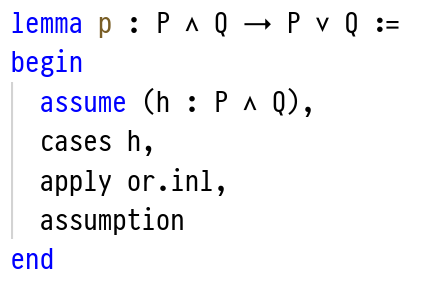
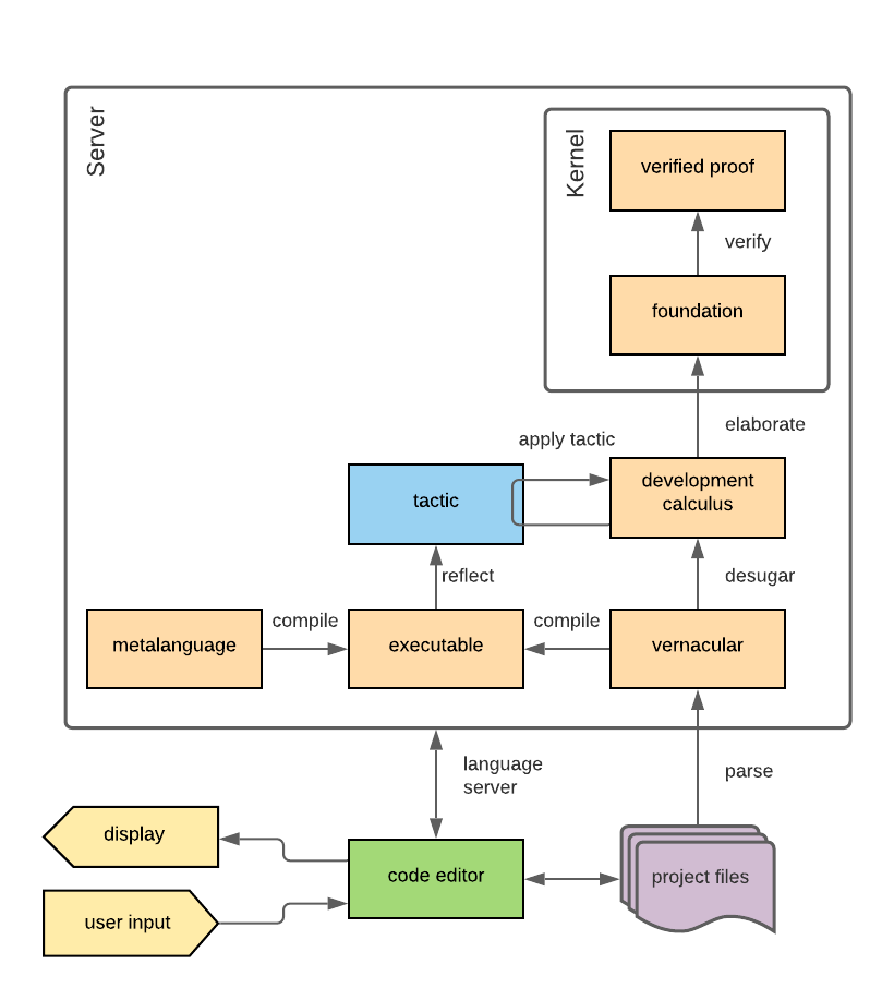
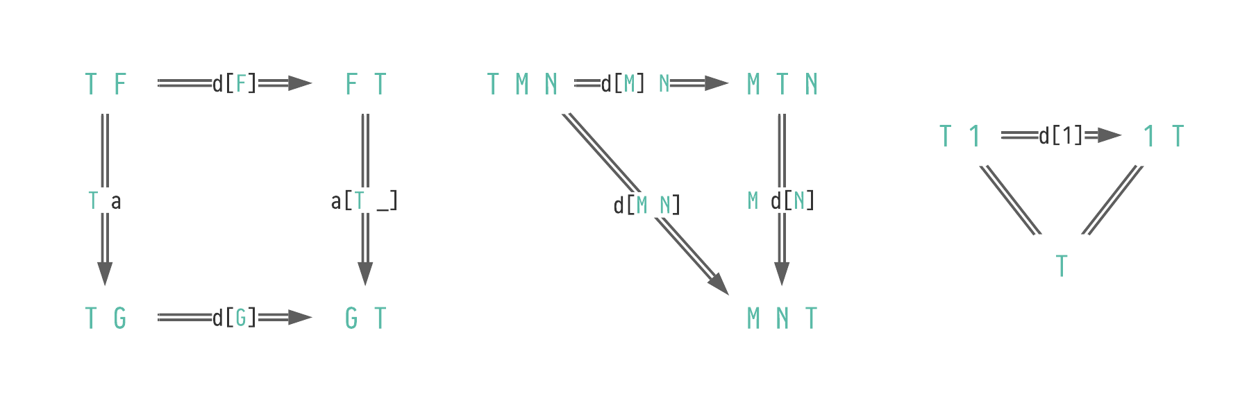
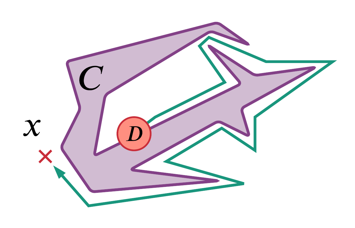
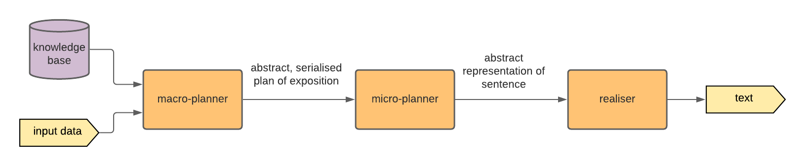
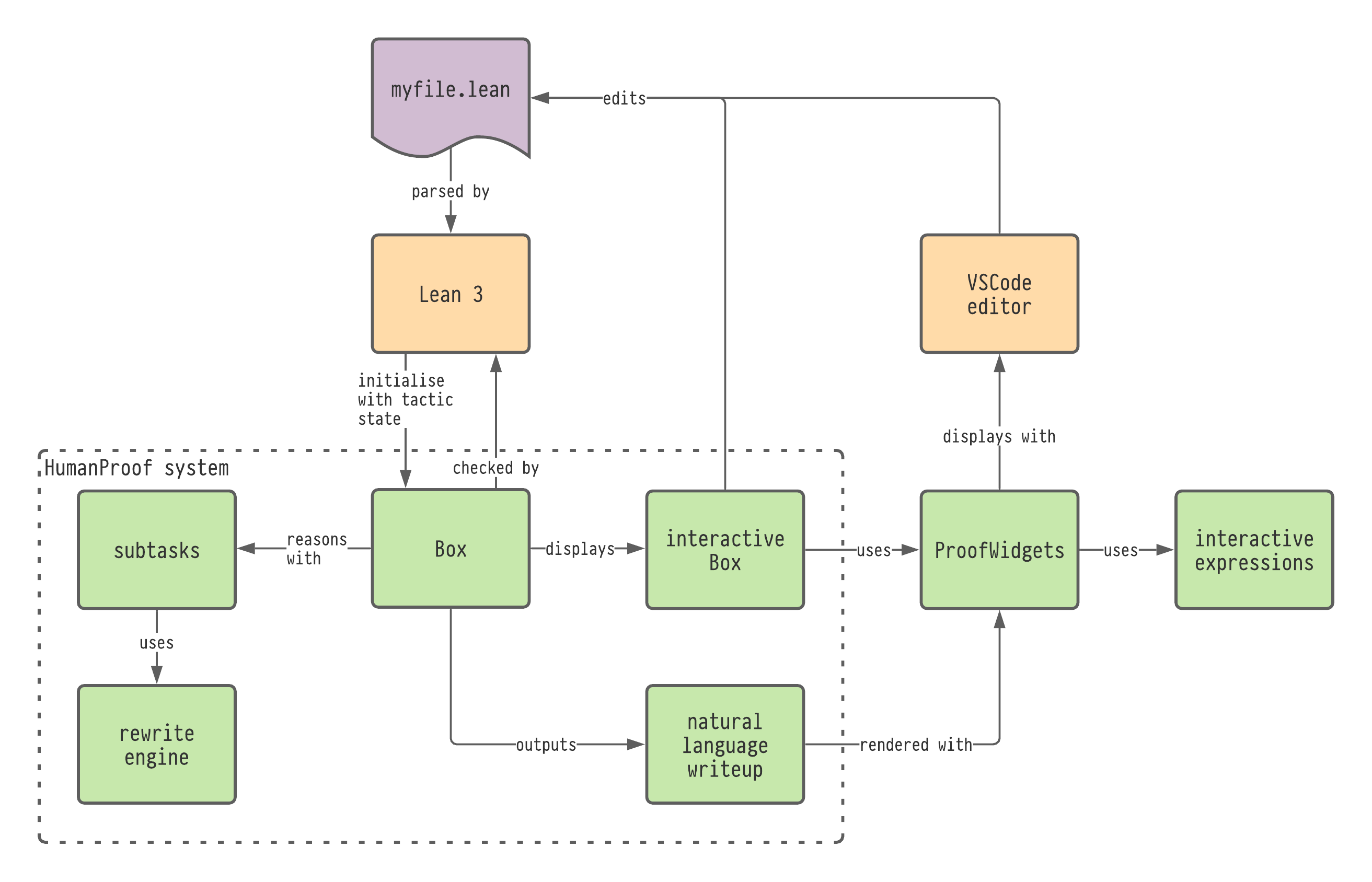
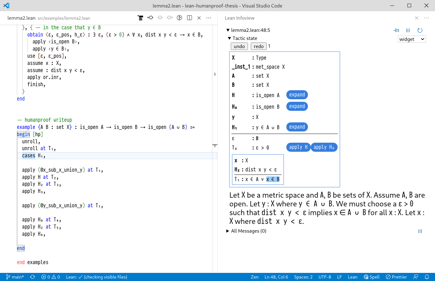
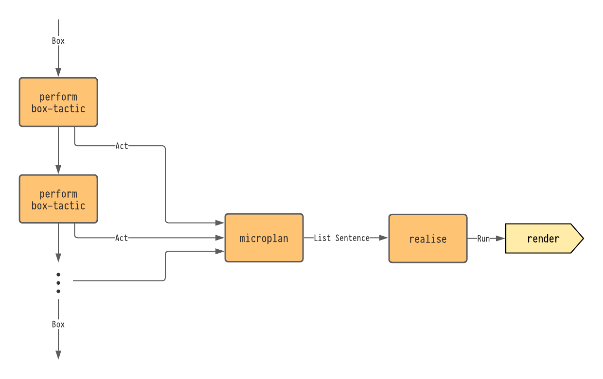
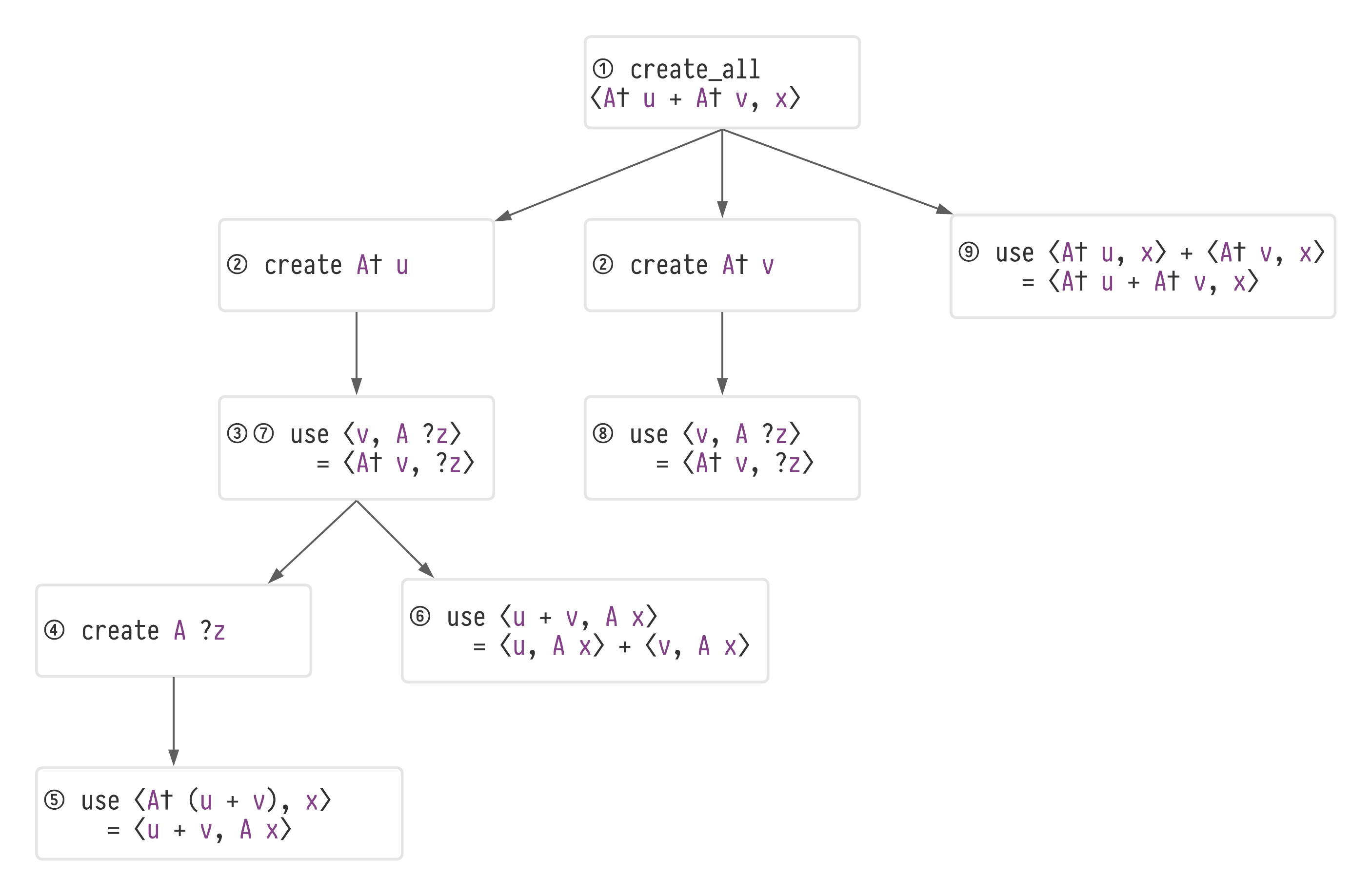
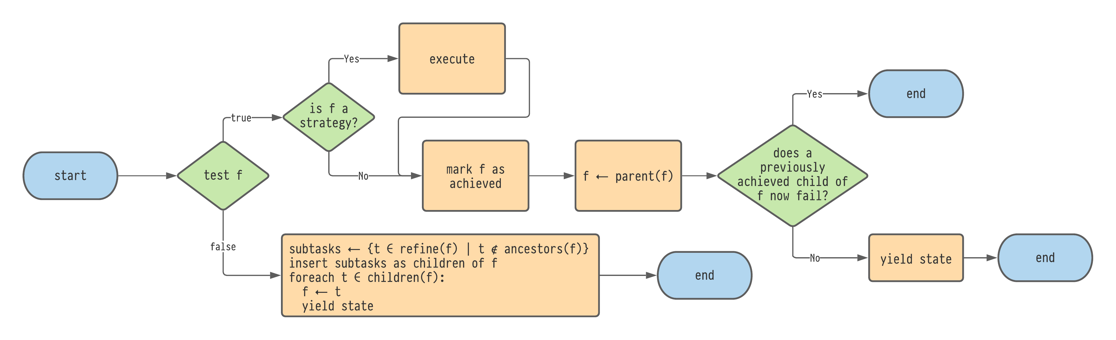


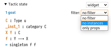

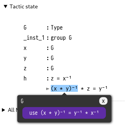
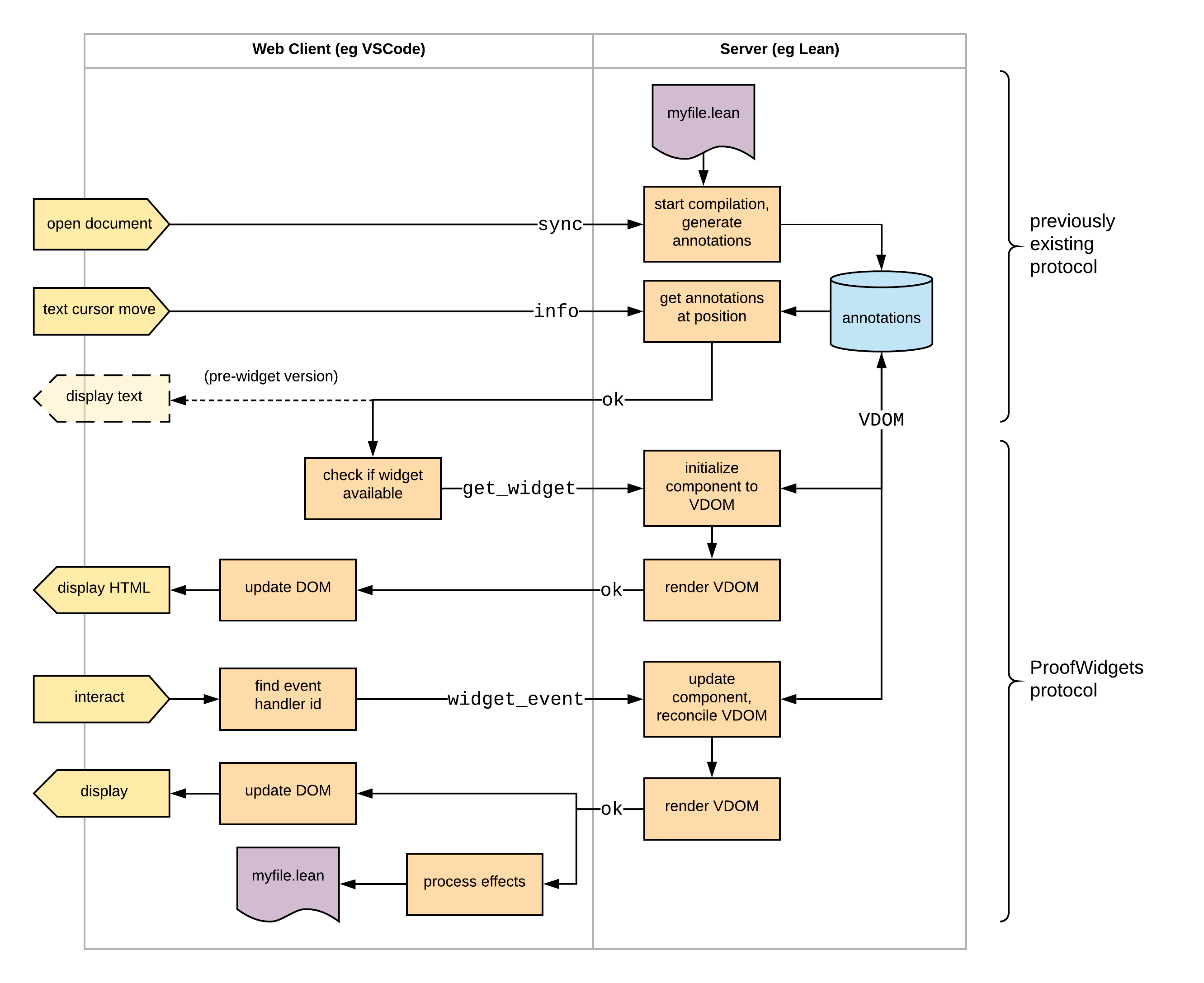
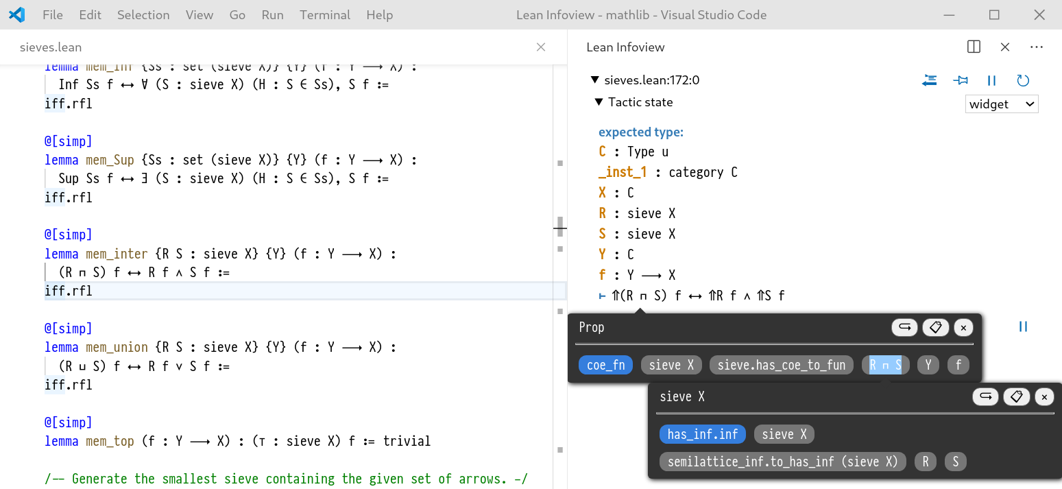


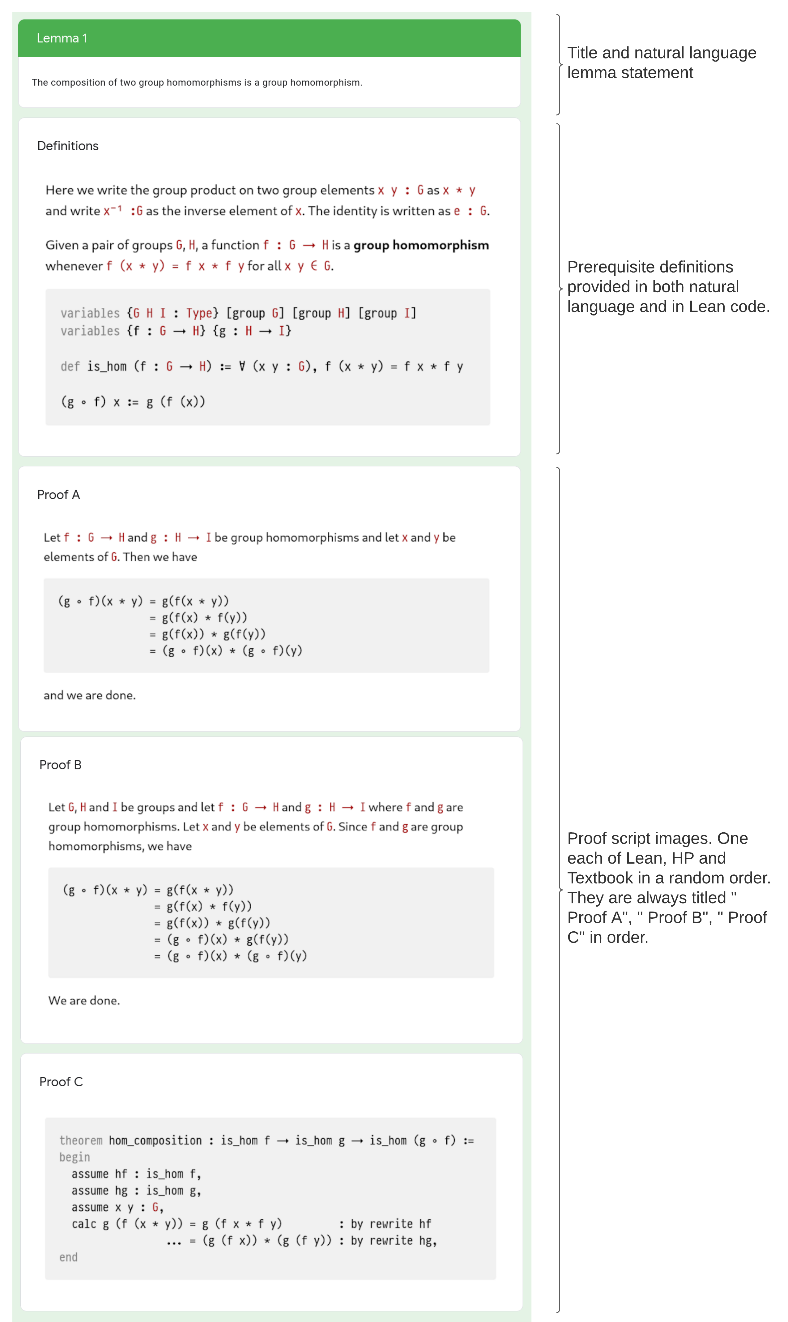

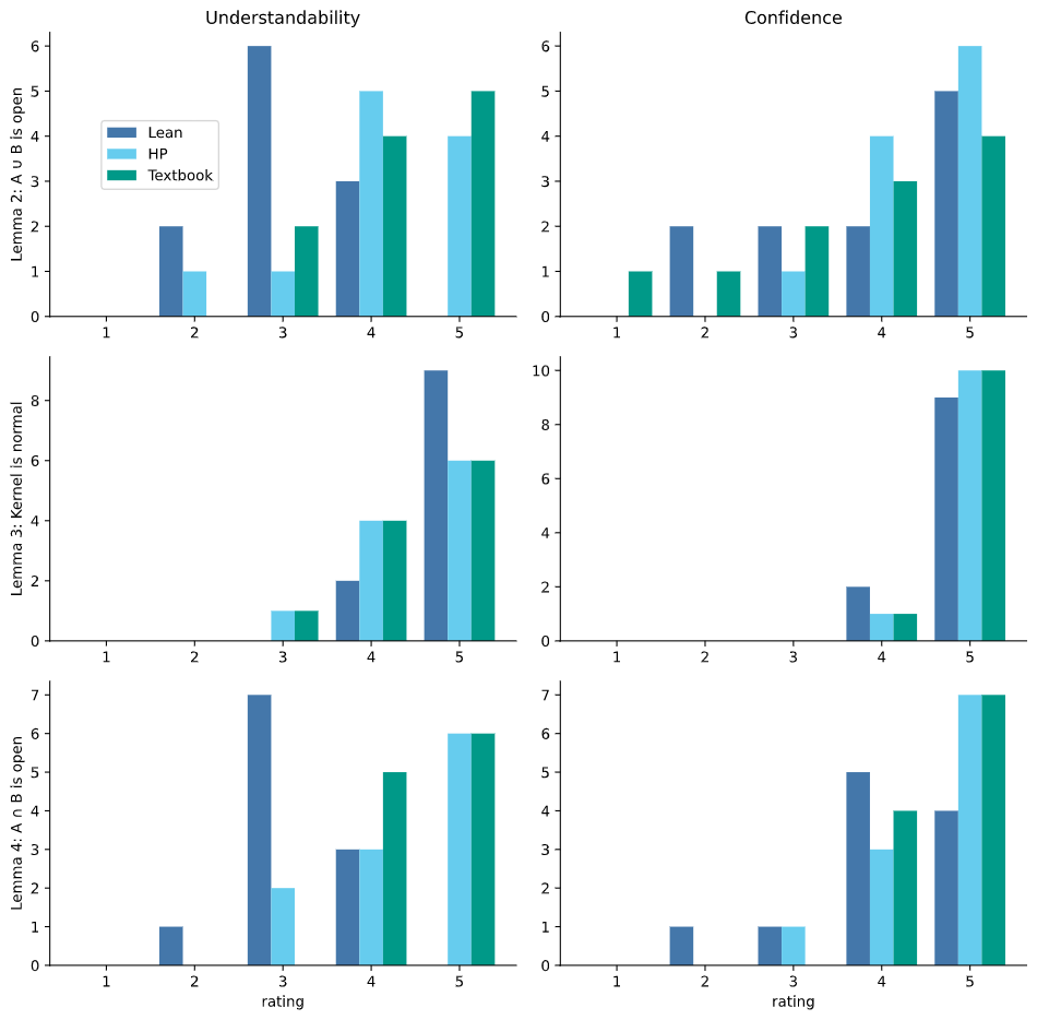
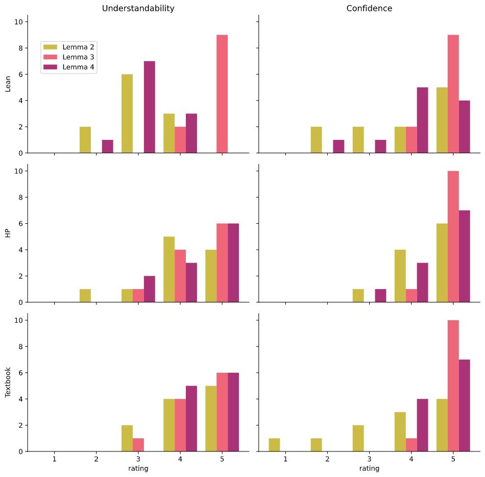
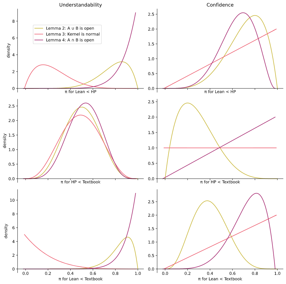
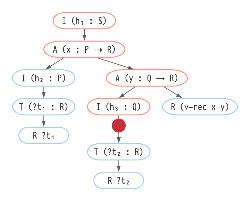
 . If you can't see this button then you may need to install the Lean extension for VSCode, consult the